22  Introduction to Bayesian Inference

22.1 Lecture

Amazing beasties and crazy animals

Dream pet dragon

need to add stuff here

22.1.1 Bayes’ theorem

First, let’s review the theorem. Mathematically, it says how to convert one conditional probability into another one.

\[ P(B \mid A) = \frac{ P(A \mid B) * P(B)}{P(A)} \]

The formula becomes more interesting in the context of statistical modeling. We have some model that describes a data-generating process and we have some observed data, but we want to estimate some unknown model parameters. In that case, the formula reads like:

\[ P(\text{hypothesis} \mid \text{data}) = \frac{ P(\text{data} \mid \text{hypothesis}) * P(\text{hypothesis})}{P(\text{data})} \]

These terms have conventional names:

\[ \text{posterior} = \frac{ \text{likelihood} * \text{prior}}{\text{evidence}} \]

Prior and posterior describe when information is obtained: what we know pre-data is our prior information, and what we learn post-data is the updated information (“posterior”).

The likelihood in the equation says how likely the data is given the model parameters. I think of it as fit: How well do the parameters fit the data? Classical regression’s line of best fit is the maximum likelihood line. The likelihood also encompasses the data-generating process behind the model. For example, if we assume that the observed data is normally distributed, then we evaluate the likelihood by using the normal probability density function. You don’t need to know what that last sentence means. What’s important is that the likelihood contains our built-in assumptions about how the data is distributed.

The evidence (sometimes called average likelihood) is hareder to grasp. I am not sure how to describe it in an intuitive way. It’s there to make sure the math works out so that the posterior probabilities sum to 1. Some presentations of Bayes’ theorem gloss over it and I am not the exception 😄. The important thing to note is that the posterior is proportional to the likelihood and prior information.

\[ \text{posterior information} \propto \text{likelihood of data} * \text{prior information} \]

So simply put, you update your prior information in proportion to how well it fits the observed data. So essentially you are doing that on a daily basis for everything except when you ar doing frequentist stats 😄.

Bayesian Triptych

Warning

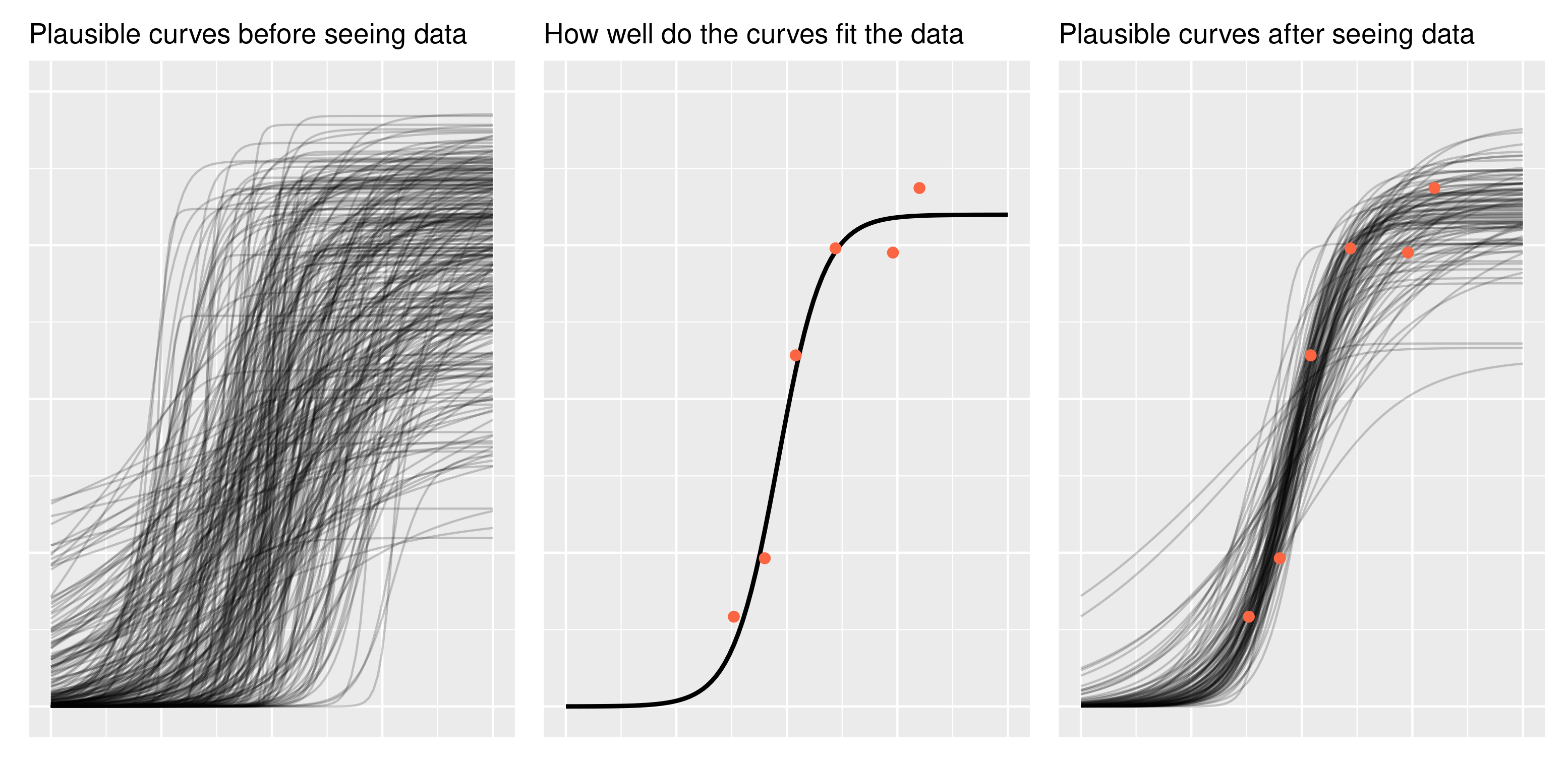
A word of encouragement! The prior is an intimidating part of Bayesian statistics. It seems highly subjective, as though we are pulling numbers from thin air, and it can be overwhelming for complex models. But if we are familiar with the kind of data we are modeling, we have prior information. We can have the model simulate new observations using the prior distribution and then plot the hypothetical data. Does anything look wrong or implausible about the simulated data? If so, then we have some prior information that we can include in our model. Note that we do not evaluate the plausibility of the simulated data based on the data we have in hand (the data we want to model); that’s not

22.1.2 Intro to MCMC

We will now walk through a simple example coded in R to illustrate how an MCMC algorithm works.

Suppose you are interested in the mean heart rate is of students when asked a question in a stat course. You are not sure what the exact mean value is, but you know the values are normally distributed with a standard deviation of 15. You have observed 5 individuals to have heart rate of 104, 120,160,90,130. You could use MCMC sampling to draw samples from the target distribution. We need to specify:

1. the starting value for the chain.
2. the length of the chain. In general, more iterations will give you more accurate output.

library(coda)
library(bayesplot)

This is bayesplot version 1.11.1

- Online documentation and vignettes at mc-stan.org/bayesplot

- bayesplot theme set to bayesplot::theme_default()

   * Does _not_ affect other ggplot2 plots

   * See ?bayesplot_theme_set for details on theme setting

set.seed(170)
hr_obs <- c(104, 112, 132, 115, 110)

start_value <- 250

n_iter <- 2500 # define number of iterations

pd_mean <- numeric(n_iter) # create vector for sample values

pd_mean[1] <- start_value # define starting value

for (i in 2:n_iter) {
  proposal <- pd_mean[i - 1] + MASS::mvrnorm(1, 0, 5) # proposal
  lprop <- sum(dnorm(proposal, hr_obs, 15)) # likelihood of proposed parameter
  lprev <- sum(dnorm(pd_mean[i - 1], hr_obs, 15))
  if (lprop / lprev > runif(1)) { # if likelihood of prosposed > likehood previous accept
    # and if likelihood is lower accept with random noise
    pd_mean[i] <- proposal
  } # if true sample the proposal
  else {
    (pd_mean[i] <- pd_mean[i - 1])
  } # if false sample the current value
}
pd_mean <- as.mcmc(data.frame(mean = pd_mean))
mcmc_combo(pd_mean, combo = c("trace", "dens"))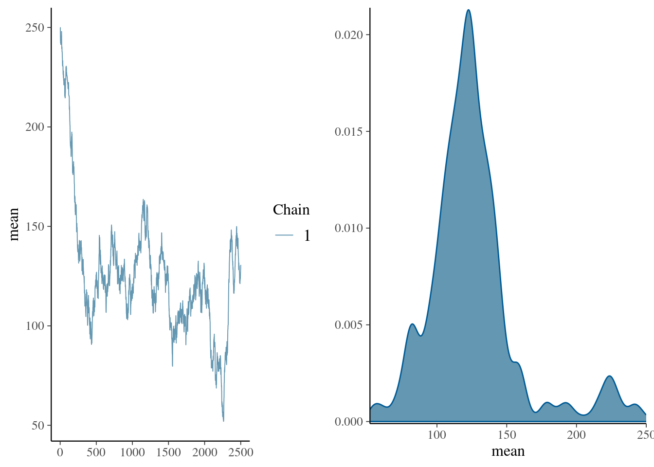

summary(pd_mean)

Iterations = 1:2500
Thinning interval = 1 
Number of chains = 1 
Sample size per chain = 2500 

1. Empirical mean and standard deviation for each variable,
   plus standard error of the mean:

          Mean             SD       Naive SE Time-series SE 
      125.8105        32.8672         0.6573        13.3046 

2. Quantiles for each variable:

  2.5%    25%    50%    75%  97.5% 
 75.53 108.03 122.19 136.12 225.46 

set.seed(170)
hr_obs <- c(104, 112, 132, 115, 110)
n_iter <- 2500 # define number of iterations

n_chain <- 3
start_value <- c(250, 100, 50)

pd_mean <- array(NA, dim = c(n_iter, n_chain, 1), dimnames = list(iter = NULL, chain = NULL, params = "beta")) # create vector for sample values

for (j in seq_len(n_chain)) {
  pd_mean[1, j, 1] <- start_value[j] # define starting value
  for (i in 2:n_iter) {
    proposal <- pd_mean[i - 1, j, 1] + MASS::mvrnorm(1, 0, 5) # proposal
    if (sum(dnorm(proposal, hr_obs, 15)) # likelihood of proposed parameter
    / sum(dnorm(pd_mean[i - 1, j, 1], hr_obs, 15)) > runif(1, 0, 1)) {
      pd_mean[i, j, 1] <- proposal
    } # if true sample the proposal
    else {
      (pd_mean[i, j, 1] <- pd_mean[i - 1, j, 1])
    } # if false sample the current value
  }
}
color_scheme_set("mix-blue-red")
mcmc_combo(pd_mean, combo = c("trace", "dens_overlay"))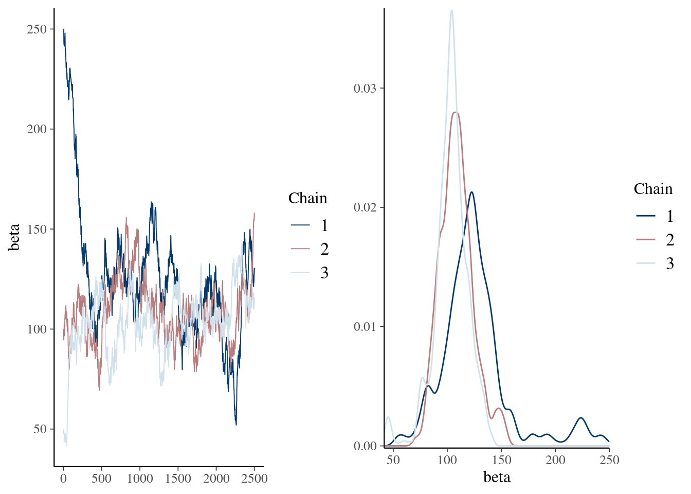

summary(pd_mean)

   Min. 1st Qu.  Median    Mean 3rd Qu.    Max. 
  41.65   99.32  109.68  112.71  122.52  250.00 

mcmc_combo(pd_mean, combo = c("trace", "dens_overlay"), n_warmup = 500)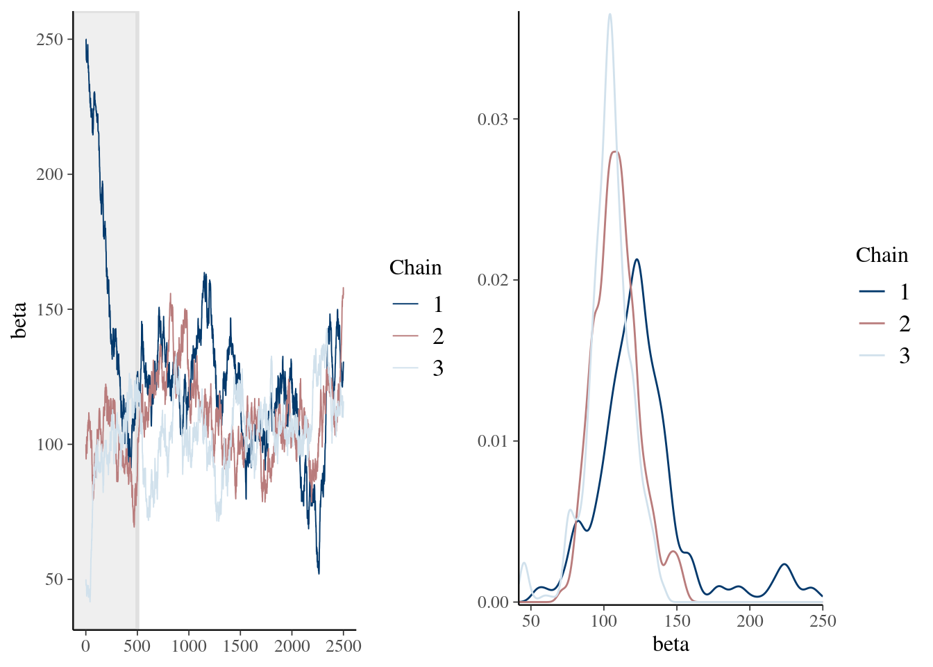

pd_burn <- pd_mean[-c(1:500), , , drop = FALSE]
summary(pd_burn)

   Min. 1st Qu.  Median    Mean 3rd Qu.    Max. 
  51.98  100.71  110.38  111.42  122.69  163.58 

mcmc_combo(pd_burn, combo = c("trace", "dens_overlay"), iter1 = 501)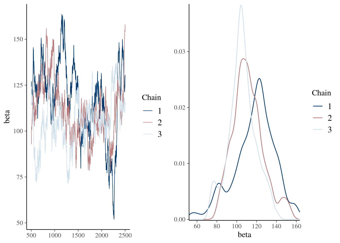

22.1.3 Inferences

22.1.3.1 Fixed effects

Easy peazy lemon squeezy just have a look at the posteriro distribution, does it overlap 0 yes or no.

talk about mean, median and mode of a distribution as well as credible intervals

22.1.3.2 Random effects

Quite a bit more harder. because constrained to be positive

• Interpreting posterior distribution
• DIC
• WAIC

22.2 Practical

In this practical, we will revisit our analysis on unicorn aggressivity. Honestly, we can use any other data with repeated measures for this exercise but I just love unicorns ❤️. However, instead of fittng the model using lmer() from the lmerTest 📦 (Kuznetsova et al. 2017), we will refit the model using 2 excellent softwares fitting models with a Bayesian approach: MCMCglmm (Hadfield 2010) and brms (Bürkner 2021).

22.2.1 R packages needed

First we load required libraries

library(lmerTest)
library(tidyverse)
library(rptR)
library(brms)
library(MCMCglmm)
library(bayesplot)

22.2.2 A refresher on unicorn ecology

The last model on unicorns was:

aggression ~ opp_size + scale(body_size, center = TRUE, scale = TRUE)
              + scale(assay_rep, scale = FALSE) + block
              + (1 | ID)

Those scaled terms are abit a sore for my eyes and way too long if we need to type them multiple times in this practical. So first let’s recode them. -

unicorns <- read.csv("data/unicorns_aggression.csv")
unicorns <- unicorns %>%
  mutate(
    body_size_sc = scale(body_size),
    assay_rep_sc = scale(assay_rep, scale = FALSE)
  )

Ok now we can fit the same model by just using:

aggression ~ opp_size + body_size_sc + assay_rep_sc + block
              + (1 | ID)

We can now fit a model using lmer(). Since we want to compare a bit REML and Bayesian aproaches, I am going to wrap the model function in a function called system.time(). This function simply estimate the user and computer time use by the function.

mer_time <- system.time(
  m_mer <- lmer(
    aggression ~ opp_size + body_size_sc + assay_rep_sc + block
      + (1 | ID),
    data = unicorns
  )
)
mer_time

   user  system elapsed 
  0.047   0.000   0.047 

summary(m_mer)

Linear mixed model fit by REML. t-tests use Satterthwaite's method [
lmerModLmerTest]
Formula: aggression ~ opp_size + body_size_sc + assay_rep_sc + block +  
    (1 | ID)
   Data: unicorns

REML criterion at convergence: 1136.5

Scaled residuals: 
     Min       1Q   Median       3Q      Max 
-2.85473 -0.62831  0.02545  0.68998  2.74064 

Random effects:
 Groups   Name        Variance Std.Dev.
 ID       (Intercept) 0.02538  0.1593  
 Residual             0.58048  0.7619  
Number of obs: 480, groups:  ID, 80

Fixed effects:
              Estimate Std. Error        df t value Pr(>|t|)    
(Intercept)    9.00181    0.03907  78.07315 230.395   <2e-16 ***
opp_size       1.05141    0.04281 396.99857  24.562   <2e-16 ***
body_size_sc   0.03310    0.03896  84.21144   0.850    0.398    
assay_rep_sc  -0.05783    0.04281 396.99857  -1.351    0.177    
block         -0.02166    0.06955 397.00209  -0.311    0.756    
---
Signif. codes:  0 '***' 0.001 '**' 0.01 '*' 0.05 '.' 0.1 ' ' 1

Correlation of Fixed Effects:
            (Intr) opp_sz bdy_s_ assy__
opp_size     0.000                     
body_siz_sc  0.000  0.000              
assay_rp_sc  0.000 -0.100  0.000       
block        0.000  0.000  0.002  0.000

Ok so it took no time at all to do it and we got our “classic” results.

22.2.3 MCMCglmm

What makes MCMCglmm so useful and powerful 💪 in ecology and for practical Bayesian people is that:

1. it is blazing fast ⏩ (for Bayesian analysis) for some models particularly models with structured covariances
2. it is fairly intuitive to code

but it also has some inconvenients:

1. it is blazing fast for Bayesian analysis meaning it is 🐌 compared to maximum likelihood approaches
2. it has some limitations in terms of functionality, distribution availability and model specifications compared to other Bayesian softwares
3. the priors, oh, the priors 😭, are a bit tricky to code and understand 🤯.

22.2.3.1 Fitting the Model

So here is how we can code the model in MCMCglmm(). It is fairly similar to lmer() except that the random effects are specified in a different argument.

mcglm_time <- system.time(
  m_mcmcglmm <- MCMCglmm(
    aggression ~ opp_size + body_size_sc + assay_rep_sc + block,
    random = ~ID,
    data = unicorns
  )
)

                       MCMC iteration = 0

                       MCMC iteration = 1000

                       MCMC iteration = 2000

                       MCMC iteration = 3000

                       MCMC iteration = 4000

                       MCMC iteration = 5000

                       MCMC iteration = 6000

                       MCMC iteration = 7000

                       MCMC iteration = 8000

                       MCMC iteration = 9000

                       MCMC iteration = 10000

                       MCMC iteration = 11000

                       MCMC iteration = 12000

                       MCMC iteration = 13000

summary(m_mcmcglmm)

 Iterations = 3001:12991
 Thinning interval  = 10
 Sample size  = 1000 

 DIC: 1128.004 

 G-structure:  ~ID

   post.mean  l-95% CI u-95% CI eff.samp
ID  0.003686 9.807e-14   0.0262    45.81

 R-structure:  ~units

      post.mean l-95% CI u-95% CI eff.samp
units    0.6044   0.5228   0.6819     1000

 Location effects: aggression ~ opp_size + body_size_sc + assay_rep_sc + block 

             post.mean l-95% CI u-95% CI eff.samp  pMCMC    
(Intercept)    9.00152  8.93150  9.07158     1000 <0.001 ***
opp_size       1.04940  0.96813  1.12946     1000 <0.001 ***
body_size_sc   0.03154 -0.03985  0.09563     1000  0.410    
assay_rep_sc  -0.05620 -0.13196  0.03546      893  0.184    
block         -0.02069 -0.16186  0.11553     1000  0.774    
---
Signif. codes:  0 '***' 0.001 '**' 0.01 '*' 0.05 '.' 0.1 ' ' 1

mcglm_time

   user  system elapsed 
  1.058   0.001   1.059 

Model is slow and not good. We need more iteration and maybe even a longer burnin, and honestly maybe better priors.

We can still take the time to have a look at the R object output from MCMCglmm(). The 2 main parts we are interrested in are:

• Sol which stand for the model solution and includes the posteriro distribution of the fixed effects
• VCV, for the variance covariance estimates, which includes the posterior distribution of all (co)variances estimates for both random effects and residual variance.

omar <- par()
par(mar = c(4, 2, 1.5, 2))
plot(m_mcmcglmm$Sol)

Posterior trace and distribution of the parameters in m_mcmcglmm using default settings

Posterior trace and distribution of the parameters in m_mcmcglmm using default settings

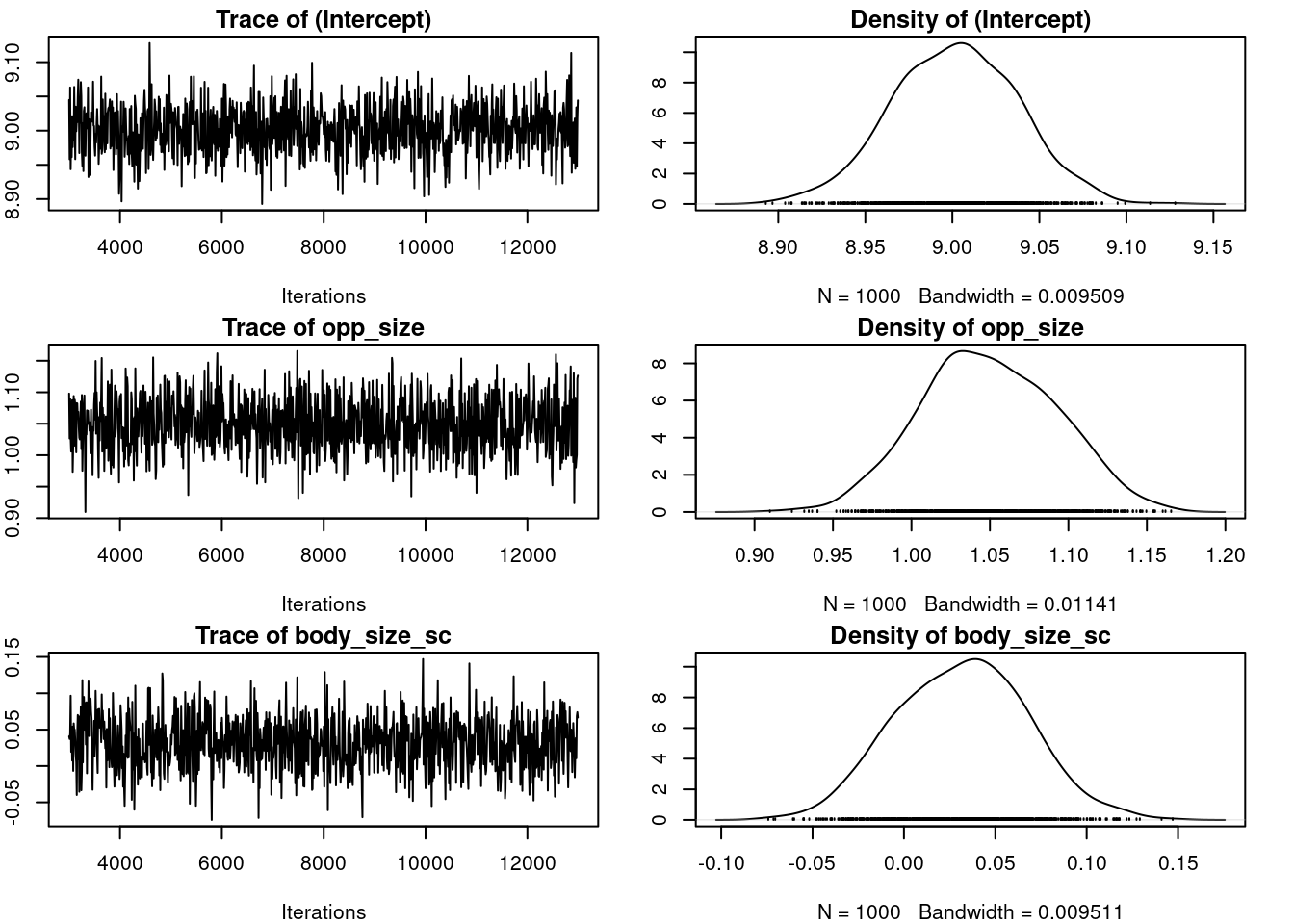
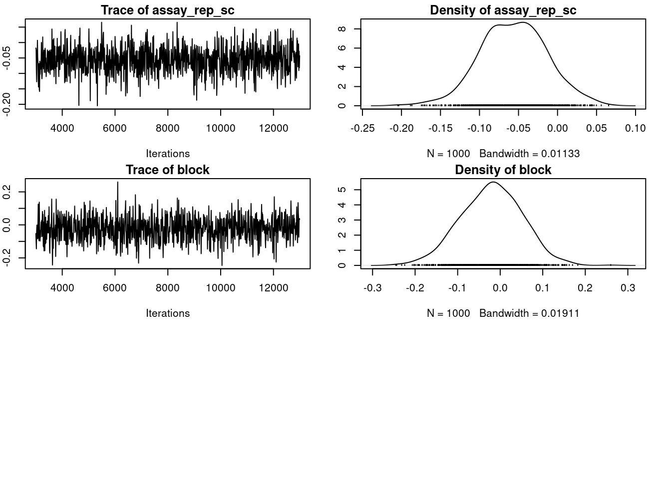
plot(m_mcmcglmm$VCV)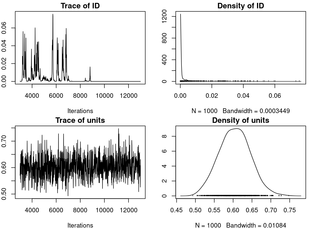

Posterior trace and distribution of the parameters in m_mcmcglmm using default settings

par(omar)
autocorr.diag(m_mcmcglmm$VCV)

               ID       units
Lag 0   1.0000000  1.00000000
Lag 10  0.8042405 -0.02074155
Lag 50  0.4807583 -0.04264317
Lag 100 0.1951356  0.04422296
Lag 500 0.1254589  0.04401956

Talk about autocorrelation, mixing, convergence and priors here

n_samp <- 1000
thin <- 500
burnin <- 20000
mcglm_time <- system.time(
  m_mcmcglmm <- MCMCglmm(
    aggression ~ opp_size + body_size_sc + assay_rep_sc + block,
    random = ~ID,
    data = unicorns,
    nitt = n_samp * thin + burnin, thin = thin, burnin = burnin,
    verbose = FALSE,
    prior = list(
      R = list(V = 1, nu = 0.002),
      G = list(
        G1 = list(V = 1, nu = 0.002)
      )
    )
  )
)
summary(m_mcmcglmm)

 Iterations = 20001:519501
 Thinning interval  = 500
 Sample size  = 1000 

 DIC: 1126.66 

 G-structure:  ~ID

   post.mean  l-95% CI u-95% CI eff.samp
ID   0.01987 0.0002904  0.05458     1000

 R-structure:  ~units

      post.mean l-95% CI u-95% CI eff.samp
units    0.5917   0.5188   0.6763     1000

 Location effects: aggression ~ opp_size + body_size_sc + assay_rep_sc + block 

             post.mean l-95% CI u-95% CI eff.samp  pMCMC    
(Intercept)    9.00136  8.92221  9.07383     1000 <0.001 ***
opp_size       1.05363  0.96382  1.13650     1000 <0.001 ***
body_size_sc   0.03373 -0.03781  0.10686     1000  0.396    
assay_rep_sc  -0.05861 -0.14186  0.02882     1000  0.182    
block         -0.02709 -0.16061  0.11441     1000  0.698    
---
Signif. codes:  0 '***' 0.001 '**' 0.01 '*' 0.05 '.' 0.1 ' ' 1

mcglm_time

   user  system elapsed 
 55.513   0.002  55.569 

evaluate model here

omar <- par()
par(mar = c(4, 2, 1.5, 2))
plot(m_mcmcglmm$Sol)

Posterior trace and distribution of the paremeters in m_mcmcglmm with better settings

Posterior trace and distribution of the paremeters in m_mcmcglmm with better settings

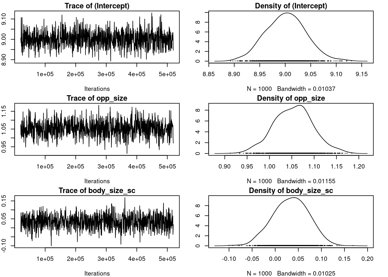
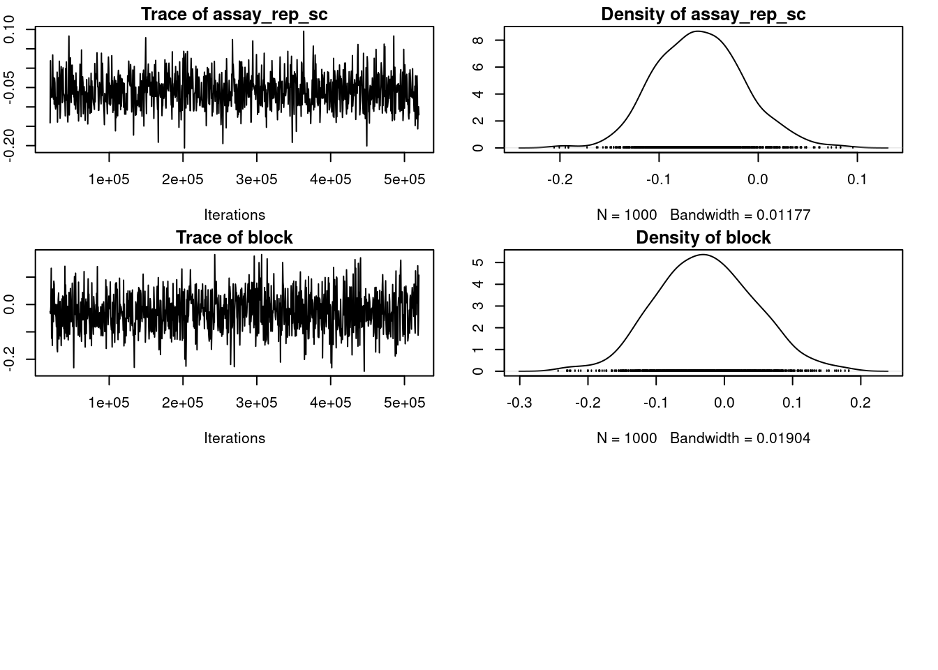
plot(m_mcmcglmm$VCV)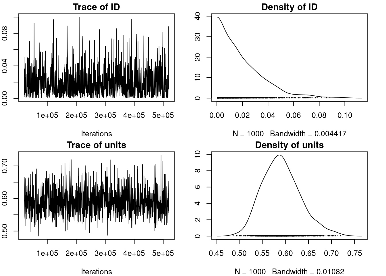

Posterior trace and distribution of the paremeters in m_mcmcglmm with better settings

par(omar)
autocorr.diag(m_mcmcglmm$VCV)

                    ID        units
Lag 0      1.000000000  1.000000000
Lag 500    0.013876043 -0.044235206
Lag 2500   0.026120260 -0.048012241
Lag 5000  -0.049357725  0.021158672
Lag 25000  0.002544256 -0.003722595

22.2.4 Inferences

22.2.4.1 Fixed effects

Easy peazy lemon squeezy just have a look at the posterior distribution, does it overlap 0 yes or no.

posterior.mode(m_mcmcglmm$Sol)

 (Intercept)     opp_size body_size_sc assay_rep_sc        block 
  9.00632282   1.07353252   0.03500916  -0.04048582  -0.03276275 

HPDinterval(m_mcmcglmm$Sol)

                   lower      upper
(Intercept)   8.92221005 9.07383400
opp_size      0.96382086 1.13649873
body_size_sc -0.03781276 0.10685606
assay_rep_sc -0.14185602 0.02882443
block        -0.16060691 0.11440706
attr(,"Probability")
[1] 0.95

22.2.4.2 Random effects

Quite a bit more harder. because constrained to be positive

posterior.mode(m_mcmcglmm$VCV)

        ID      units 
0.00096263 0.59129362 

HPDinterval(m_mcmcglmm$VCV)

             lower      upper
ID    0.0002903938 0.05458376
units 0.5188238599 0.67634529
attr(,"Probability")
[1] 0.95

22.2.5 brms

brms is an acronym for Bayesian Regression Models using ‘Stan’ (Bürkner 2021). It is a package developed to fit regression models with a Bayesian approach using the amazing stan software (Stan Development Team 2021).

What makes brms so useful and powerful 💪 in ecology is that:

1. it is really intuitive to code (same syntax as glmer())
2. it is incredibly flexible since it is essentially a front end for stan via its rstan interface (Stan Development Team 2024)

but with great powers come great responsability 🕷️

brm_time <- system.time(
  m_brm <- brm(
    aggression ~ opp_size + body_size_sc + assay_rep_sc + block
      + (1 | ID),
    data = unicorns, iter = 4750, warmup = 1000, thin = 15, cores = 4
    # refresh = 0
  )
)

Compiling Stan program...

Start sampling

brm_time

   user  system elapsed 
 83.111   4.528  75.310 

summary(m_brm)

 Family: gaussian 
  Links: mu = identity; sigma = identity 
Formula: aggression ~ opp_size + body_size_sc + assay_rep_sc + block + (1 | ID) 
   Data: unicorns (Number of observations: 480) 
  Draws: 4 chains, each with iter = 4750; warmup = 1000; thin = 15;
         total post-warmup draws = 1000

Multilevel Hyperparameters:
~ID (Number of levels: 80) 
              Estimate Est.Error l-95% CI u-95% CI Rhat Bulk_ESS Tail_ESS
sd(Intercept)     0.14      0.07     0.01     0.28 1.00     1037      973

Regression Coefficients:
             Estimate Est.Error l-95% CI u-95% CI Rhat Bulk_ESS Tail_ESS
Intercept        9.00      0.04     8.92     9.08 1.00     1005     1024
opp_size         1.05      0.04     0.97     1.14 1.00      855      819
body_size_sc     0.03      0.04    -0.04     0.11 1.00      957      938
assay_rep_sc    -0.06      0.05    -0.15     0.03 1.00     1047     1038
block           -0.02      0.07    -0.14     0.12 1.01      999      973

Further Distributional Parameters:
      Estimate Est.Error l-95% CI u-95% CI Rhat Bulk_ESS Tail_ESS
sigma     0.77      0.03     0.72     0.83 1.01     1039      950

Draws were sampled using sampling(NUTS). For each parameter, Bulk_ESS
and Tail_ESS are effective sample size measures, and Rhat is the potential
scale reduction factor on split chains (at convergence, Rhat = 1).

mcmc_acf_bar(m_brm, regex_pars = c("sd"))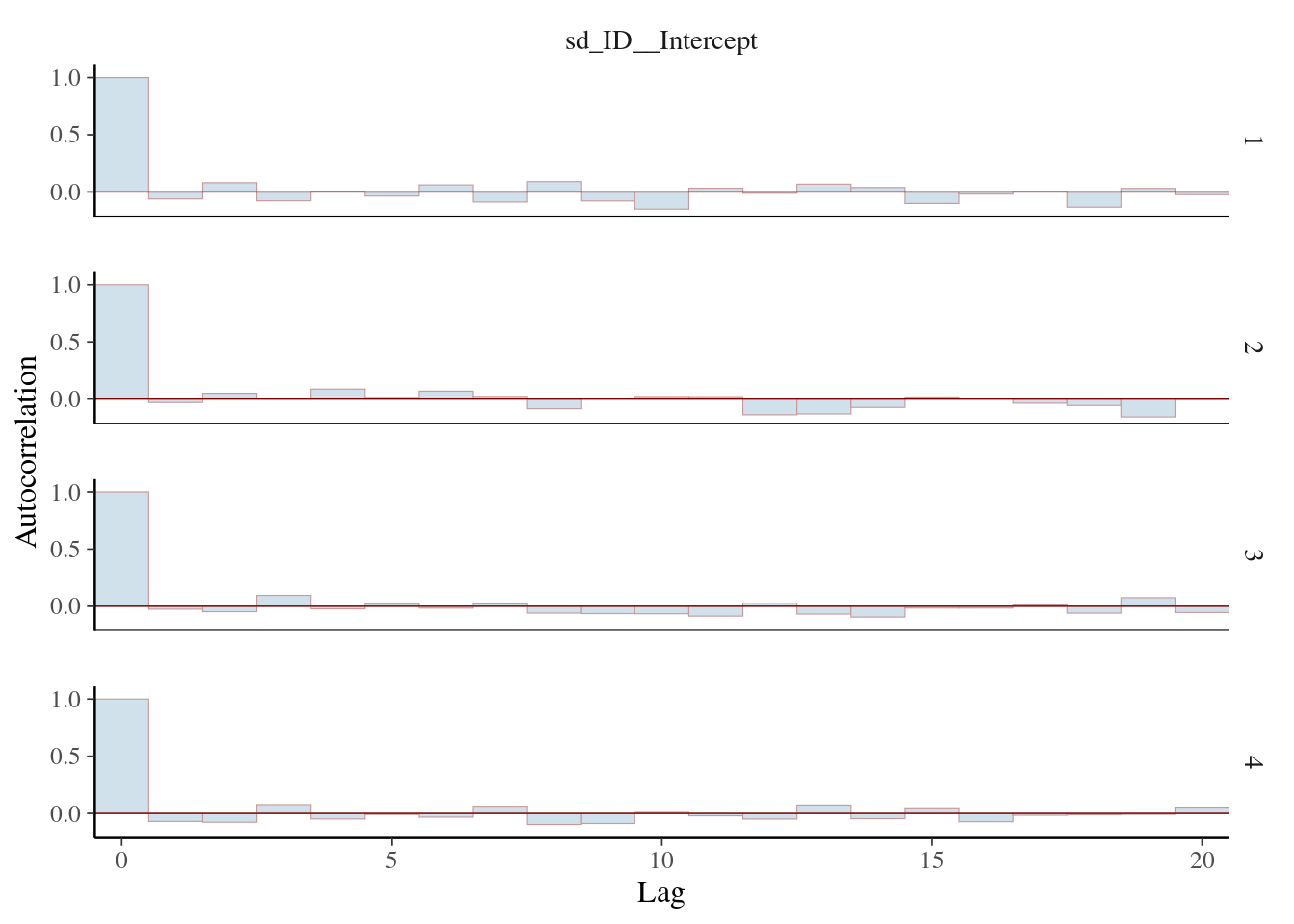

Autocorrelation in the chain for variance parameters in model m_brm

22.2.5.1 Hunder the hood

have a look at the stan code

stancode(m_brm)

// generated with brms 2.21.0
functions {
}
data {
  int<lower=1> N;  // total number of observations
  vector[N] Y;  // response variable
  int<lower=1> K;  // number of population-level effects
  matrix[N, K] X;  // population-level design matrix
  int<lower=1> Kc;  // number of population-level effects after centering
  // data for group-level effects of ID 1
  int<lower=1> N_1;  // number of grouping levels
  int<lower=1> M_1;  // number of coefficients per level
  array[N] int<lower=1> J_1;  // grouping indicator per observation
  // group-level predictor values
  vector[N] Z_1_1;
  int prior_only;  // should the likelihood be ignored?
}
transformed data {
  matrix[N, Kc] Xc;  // centered version of X without an intercept
  vector[Kc] means_X;  // column means of X before centering
  for (i in 2:K) {
    means_X[i - 1] = mean(X[, i]);
    Xc[, i - 1] = X[, i] - means_X[i - 1];
  }
}
parameters {
  vector[Kc] b;  // regression coefficients
  real Intercept;  // temporary intercept for centered predictors
  real<lower=0> sigma;  // dispersion parameter
  vector<lower=0>[M_1] sd_1;  // group-level standard deviations
  array[M_1] vector[N_1] z_1;  // standardized group-level effects
}
transformed parameters {
  vector[N_1] r_1_1;  // actual group-level effects
  real lprior = 0;  // prior contributions to the log posterior
  r_1_1 = (sd_1[1] * (z_1[1]));
  lprior += student_t_lpdf(Intercept | 3, 8.9, 2.5);
  lprior += student_t_lpdf(sigma | 3, 0, 2.5)
    - 1 * student_t_lccdf(0 | 3, 0, 2.5);
  lprior += student_t_lpdf(sd_1 | 3, 0, 2.5)
    - 1 * student_t_lccdf(0 | 3, 0, 2.5);
}
model {
  // likelihood including constants
  if (!prior_only) {
    // initialize linear predictor term
    vector[N] mu = rep_vector(0.0, N);
    mu += Intercept;
    for (n in 1:N) {
      // add more terms to the linear predictor
      mu[n] += r_1_1[J_1[n]] * Z_1_1[n];
    }
    target += normal_id_glm_lpdf(Y | Xc, mu, b, sigma);
  }
  // priors including constants
  target += lprior;
  target += std_normal_lpdf(z_1[1]);
}
generated quantities {
  // actual population-level intercept
  real b_Intercept = Intercept - dot_product(means_X, b);
}

22.2.5.2 using shiny

launch_shinystan(m_brm)

Shinystan interface

22.2.6 Inferences

22.2.6.1 Fixed effects

summary(m_brm)

 Family: gaussian 
  Links: mu = identity; sigma = identity 
Formula: aggression ~ opp_size + body_size_sc + assay_rep_sc + block + (1 | ID) 
   Data: unicorns (Number of observations: 480) 
  Draws: 4 chains, each with iter = 4750; warmup = 1000; thin = 15;
         total post-warmup draws = 1000

Multilevel Hyperparameters:
~ID (Number of levels: 80) 
              Estimate Est.Error l-95% CI u-95% CI Rhat Bulk_ESS Tail_ESS
sd(Intercept)     0.14      0.07     0.01     0.28 1.00     1037      973

Regression Coefficients:
             Estimate Est.Error l-95% CI u-95% CI Rhat Bulk_ESS Tail_ESS
Intercept        9.00      0.04     8.92     9.08 1.00     1005     1024
opp_size         1.05      0.04     0.97     1.14 1.00      855      819
body_size_sc     0.03      0.04    -0.04     0.11 1.00      957      938
assay_rep_sc    -0.06      0.05    -0.15     0.03 1.00     1047     1038
block           -0.02      0.07    -0.14     0.12 1.01      999      973

Further Distributional Parameters:
      Estimate Est.Error l-95% CI u-95% CI Rhat Bulk_ESS Tail_ESS
sigma     0.77      0.03     0.72     0.83 1.01     1039      950

Draws were sampled using sampling(NUTS). For each parameter, Bulk_ESS
and Tail_ESS are effective sample size measures, and Rhat is the potential
scale reduction factor on split chains (at convergence, Rhat = 1).

mcmc_plot(m_brm, regex_pars = "b_")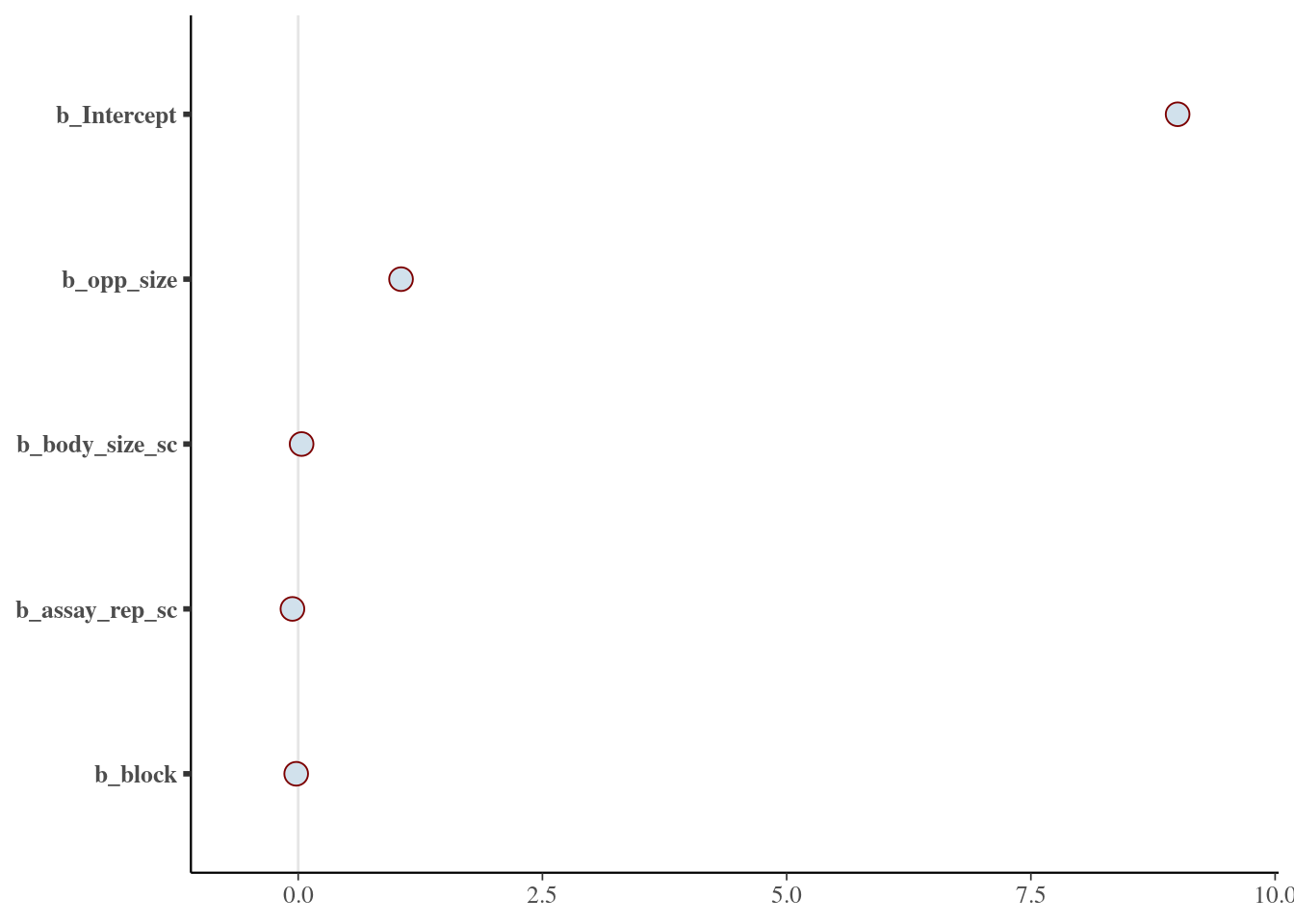

Fixed effect estimates (with 95% credible intervals) from model m_brm

22.2.6.2 Random effects

summary(m_brm)

 Family: gaussian 
  Links: mu = identity; sigma = identity 
Formula: aggression ~ opp_size + body_size_sc + assay_rep_sc + block + (1 | ID) 
   Data: unicorns (Number of observations: 480) 
  Draws: 4 chains, each with iter = 4750; warmup = 1000; thin = 15;
         total post-warmup draws = 1000

Multilevel Hyperparameters:
~ID (Number of levels: 80) 
              Estimate Est.Error l-95% CI u-95% CI Rhat Bulk_ESS Tail_ESS
sd(Intercept)     0.14      0.07     0.01     0.28 1.00     1037      973

Regression Coefficients:
             Estimate Est.Error l-95% CI u-95% CI Rhat Bulk_ESS Tail_ESS
Intercept        9.00      0.04     8.92     9.08 1.00     1005     1024
opp_size         1.05      0.04     0.97     1.14 1.00      855      819
body_size_sc     0.03      0.04    -0.04     0.11 1.00      957      938
assay_rep_sc    -0.06      0.05    -0.15     0.03 1.00     1047     1038
block           -0.02      0.07    -0.14     0.12 1.01      999      973

Further Distributional Parameters:
      Estimate Est.Error l-95% CI u-95% CI Rhat Bulk_ESS Tail_ESS
sigma     0.77      0.03     0.72     0.83 1.01     1039      950

Draws were sampled using sampling(NUTS). For each parameter, Bulk_ESS
and Tail_ESS are effective sample size measures, and Rhat is the potential
scale reduction factor on split chains (at convergence, Rhat = 1).

mcmc_plot(m_brm, pars = c("sd_ID__Intercept", "sigma"))

Warning: Argument 'pars' is deprecated. Please use 'variable' instead.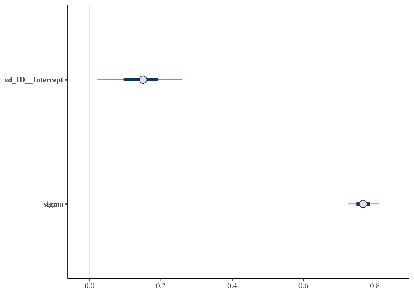

Among-individual and residual standard deviance ( with 95% credible intervals) estimated from model m_brm

22.2.7 Happy Bayesian stats

Sherlock Holmes, a truly bayesian detective

Bürkner, P.-C. 2021. Bayesian item response modeling in R with brms and Stan. Journal of Statistical Software 100:1–54.

Hadfield, J. D. 2010. MCMC methods for multi-response generalized linear mixed models: The MCMCglmm R package. Journal of Statistical Software 33:1–22.

Kuznetsova, A., P. B. Brockhoff, and R. H. B. Christensen. 2017. lmerTest package: Tests in linear mixed effects models. Journal of Statistical Software 82:1–26.

Stan Development Team. 2021. Stan modeling language users guide and reference manual, 2.26.

Stan Development Team. 2024. RStan: The R interface to Stan.