15 Generalized linear model, `glm`

15.1 Lecture

m1 <- glm(fish ~ french_captain, data = dads_joke, family = poisson)

15.1.1 Distributions

15.1.1.1 Continuous linear

Gaussian

15.1.1.2 Count data

poisson
negative binomial
quasi-poisson
generalized poisson
conway-maxwell poisson

15.1.1.3 censored distribution

15.1.1.4 zero-inflated / hurdle distribution

zero-inflated/zero-truncated poisson
censored poisson

15.1.1.5 zero-truncated distribution

15.1.1.6 zero-one-inflated distribution

see https://cran.r-project.org/web/packages/brms/vignettes/brms_families.html see alo MCMCglmm coursenotes

for help on description and to add some plots about those distribution

15.2 Practical

Warning

This section need to be severely updated

15.2.1 Logistic regression

library(tidyverse)

── Attaching core tidyverse packages ──────────────────────── tidyverse 2.0.0 ──
✔ dplyr     1.1.4     ✔ readr     2.1.5
✔ forcats   1.0.0     ✔ stringr   1.5.1
✔ ggplot2   3.5.1     ✔ tibble    3.2.1
✔ lubridate 1.9.3     ✔ tidyr     1.3.1
✔ purrr     1.0.2     
── Conflicts ────────────────────────────────────────── tidyverse_conflicts() ──
✖ dplyr::filter() masks stats::filter()
✖ dplyr::lag()    masks stats::lag()
ℹ Use the conflicted package (<http://conflicted.r-lib.org/>) to force all conflicts to become errors

library(DHARMa)

This is DHARMa 0.4.6. For overview type '?DHARMa'. For recent changes, type news(package = 'DHARMa')

library(performance)

mouflon <- read.csv("data/mouflon.csv")
mouflonc <- mouflon[order(mouflon$age),]

mouflonc$reproduction <- ifelse(mouflonc$age < 13, mouflonc$reproduction, 0)
mouflonc$reproduction <- ifelse(mouflonc$age > 4, mouflonc$reproduction, 1)

plot(reproduction ~ age, mouflonc)

plot(jitter(reproduction) ~ jitter(age), mouflonc)

bubble <- data.frame(age = rep(2:16, 2),
                     reproduction = rep(0:1, each = 15),
                     size = c(table(mouflonc$age, mouflonc$reproduction)))
bubble$size <- ifelse(bubble$size == 0 , NA, bubble$size)
 ggplot(data = bubble, aes(x = age, y = reproduction))+
 geom_point(aes(size = size*10))

Warning: Removed 7 rows containing missing values or values outside the scale range
(`geom_point()`).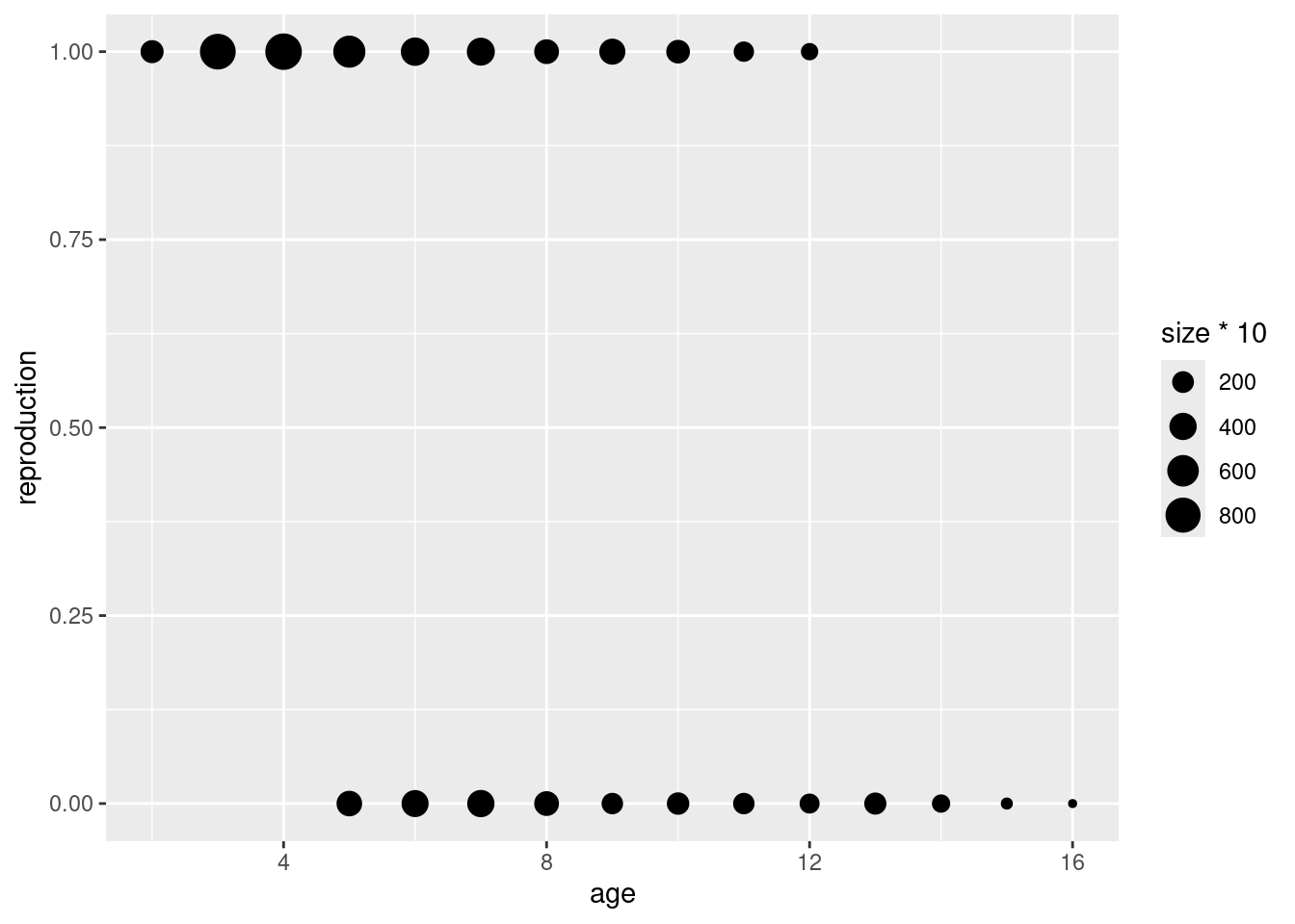

m1 <- glm(reproduction ~ age,
    data = mouflonc,
    family = binomial)
summary(m1)


Call:
glm(formula = reproduction ~ age, family = binomial, data = mouflonc)

Coefficients:
            Estimate Std. Error z value Pr(>|z|)    
(Intercept)  3.19921    0.25417   12.59   <2e-16 ***
age         -0.36685    0.03287  -11.16   <2e-16 ***
---
Signif. codes:  0 '***' 0.001 '**' 0.01 '*' 0.05 '.' 0.1 ' ' 1

(Dispersion parameter for binomial family taken to be 1)

    Null deviance: 928.86  on 715  degrees of freedom
Residual deviance: 767.51  on 714  degrees of freedom
  (4 observations deleted due to missingness)
AIC: 771.51

Number of Fisher Scoring iterations: 4

simulationOutput <- simulateResiduals(m1)
plot(simulationOutput)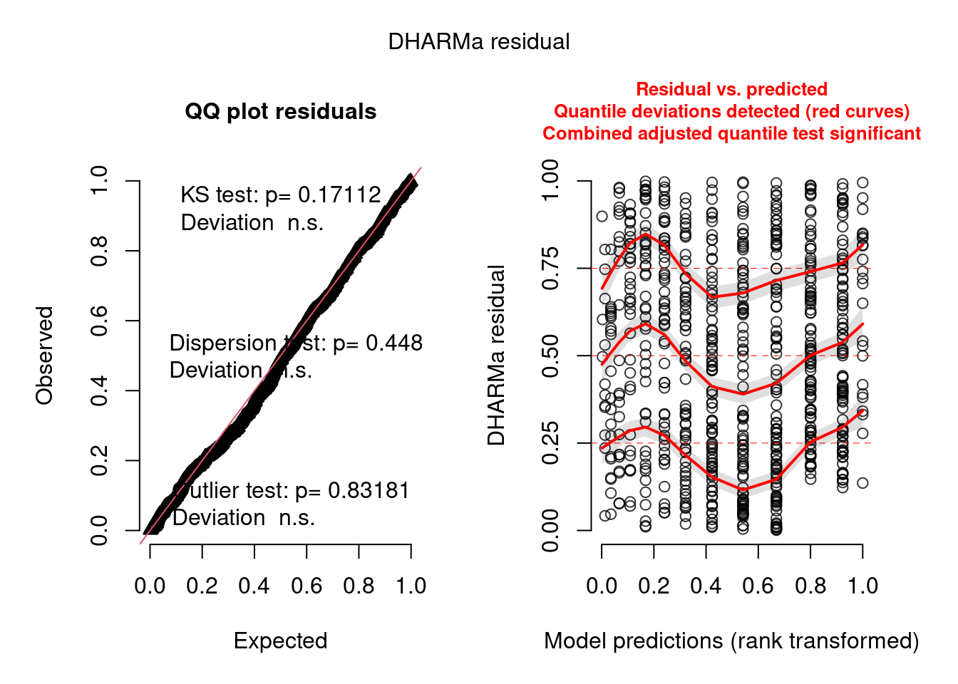

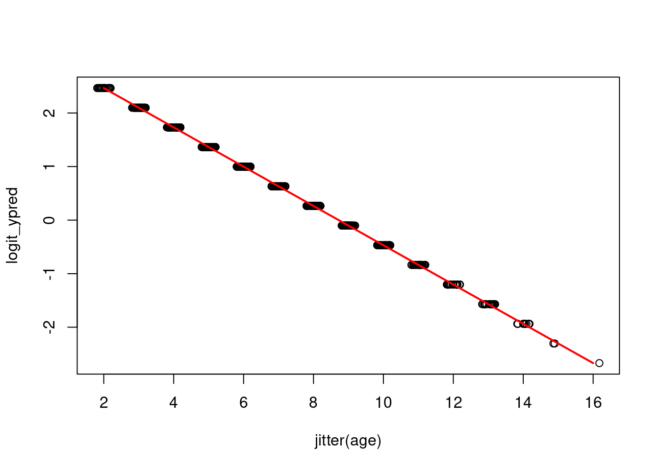
plotting the model prediction on the link (latent) scale

mouflonc$logit_ypred <- 3.19921 -0.36685 * mouflonc$age
plot(logit_ypred ~  jitter(age), mouflonc)
points(mouflonc$age, mouflonc$logit_ypred, col="red", type = "l", lwd = 2)

plotting on the observed scale

mouflonc$ypred <- exp(mouflonc$logit_ypred) / (1 + exp(mouflonc$logit_ypred)) # inverse of logit 

plot(reproduction ~  jitter(age), mouflonc)
points(mouflonc$age, mouflonc$ypred, col="red", type = "l", lwd = 2)

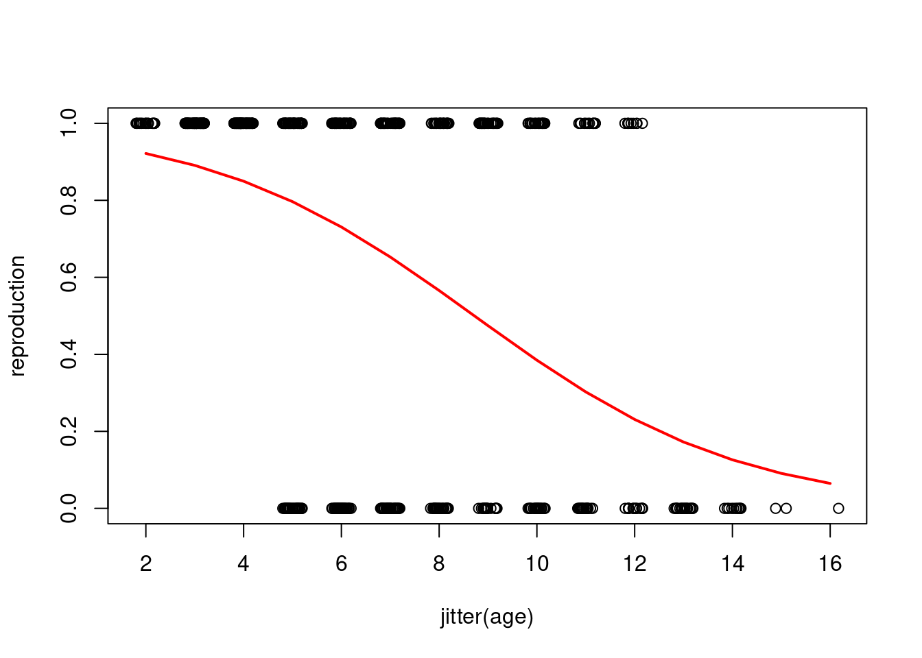
Enfin, pour se simplifier la vie, il est aussi possible de récupérer les valeurs prédites de y directement

plot(x,y)
myreg <- glm(y~x, family=binomial(link=logit))
ypredit <- myreg$fitted
o=order(x)
points(x[o],ypredit[o], col="red", type="l", lwd=2)

m2 <- glm(reproduction ~ age + mass_sept + as.factor(sex_lamb) + mass_gain + density + temp,
    data = mouflon,
    family = binomial)

summary(m2)


Call:
glm(formula = reproduction ~ age + mass_sept + as.factor(sex_lamb) + 
    mass_gain + density + temp, family = binomial, data = mouflon)

Coefficients:
                      Estimate Std. Error z value Pr(>|z|)    
(Intercept)           1.622007   1.943242   0.835 0.403892    
age                  -0.148567   0.033597  -4.422 9.78e-06 ***
mass_sept             0.029878   0.016815   1.777 0.075590 .  
as.factor(sex_lamb)1 -0.428169   0.166156  -2.577 0.009969 ** 
mass_gain            -0.094828   0.026516  -3.576 0.000348 ***
density              -0.018132   0.003518  -5.154 2.55e-07 ***
temp                  0.037244   0.138712   0.269 0.788313    
---
Signif. codes:  0 '***' 0.001 '**' 0.01 '*' 0.05 '.' 0.1 ' ' 1

(Dispersion parameter for binomial family taken to be 1)

    Null deviance: 916.06  on 674  degrees of freedom
Residual deviance: 845.82  on 668  degrees of freedom
  (45 observations deleted due to missingness)
AIC: 859.82

Number of Fisher Scoring iterations: 4

check_model(m2)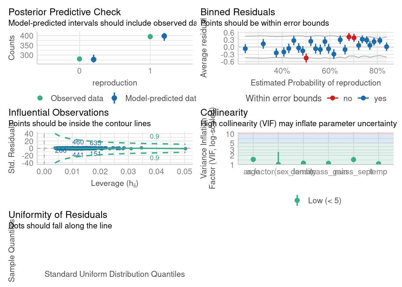

simulationOutput <- simulateResiduals(m2)
plot(simulationOutput)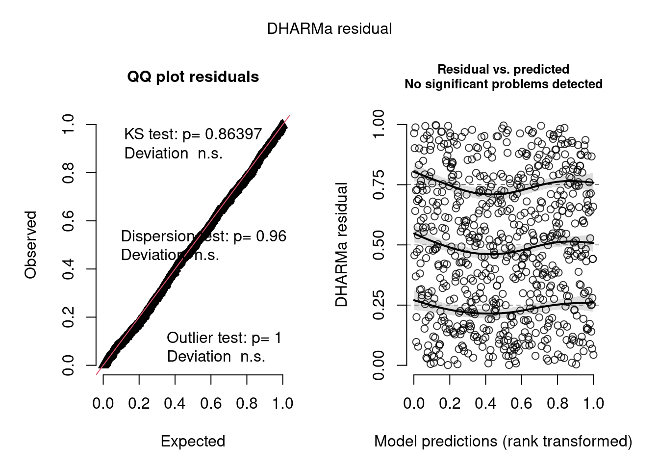

15.2.1.1 previous offspring sex effect

pred.data <- data.frame(
  age = mean(mouflon$age),
  mass_sept = mean(mouflon$mass_sept),
  sex_lamb = c(0,1),
  mass_gain = mean(mouflon$mass_gain),
  density = mean(mouflon$density),
  temp = mean(mouflon$temp, na.rm =TRUE))

  predict(m2, newdata = pred.data)

        1         2 
0.6225895 0.1944205

15.2.2 Poisson regression

data on galapagos islands species richness model of total number of species model of proportion of native model of density of species

Fit 3 models - model of total number of species - model of proportion of endemics to total - model of species density

  hist(rpois(10000,3))

#
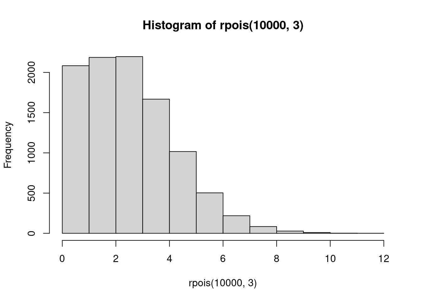
 gala <- read.delim2("data/gala.txt")
 plot(Species ~ Area, gala)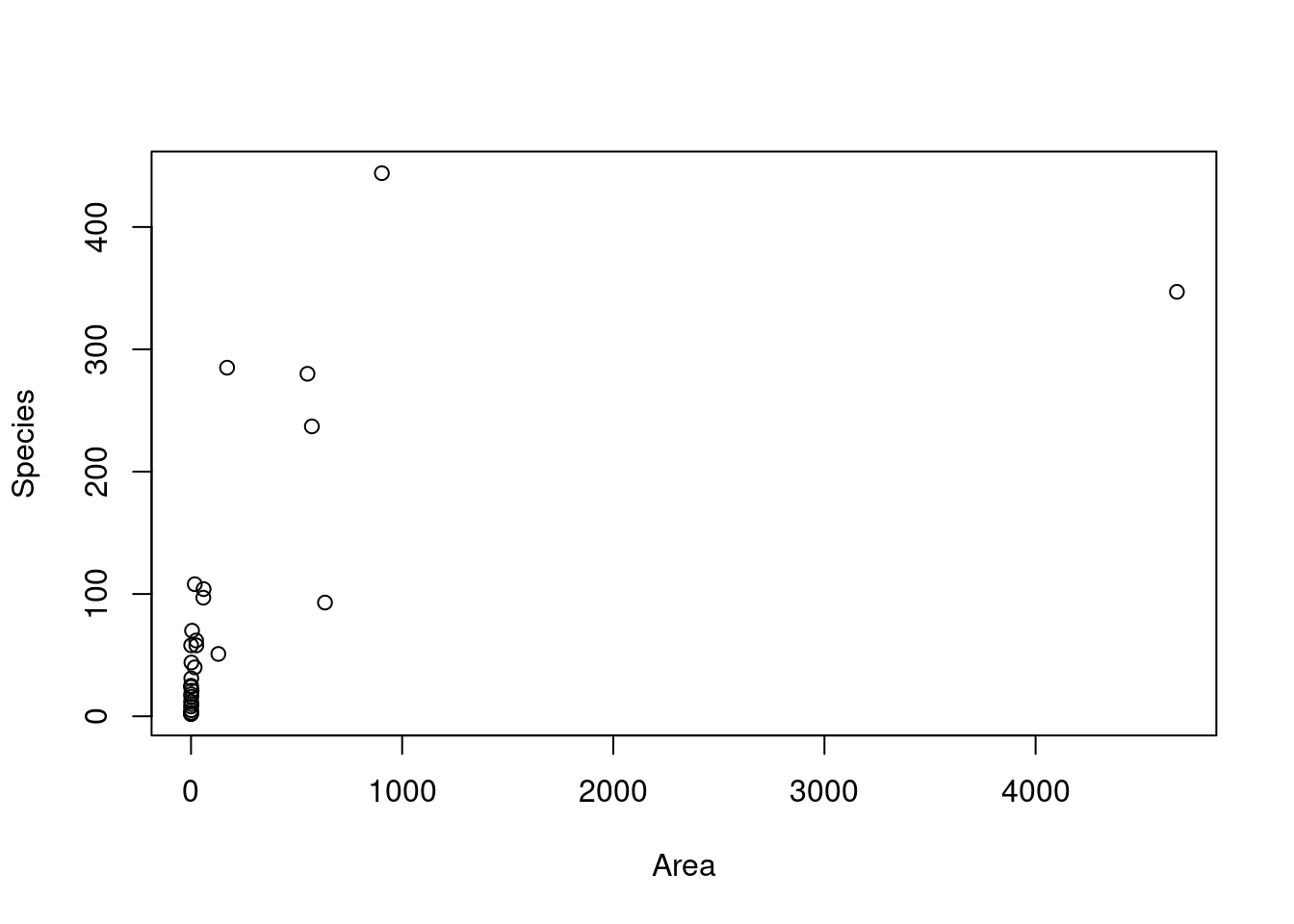

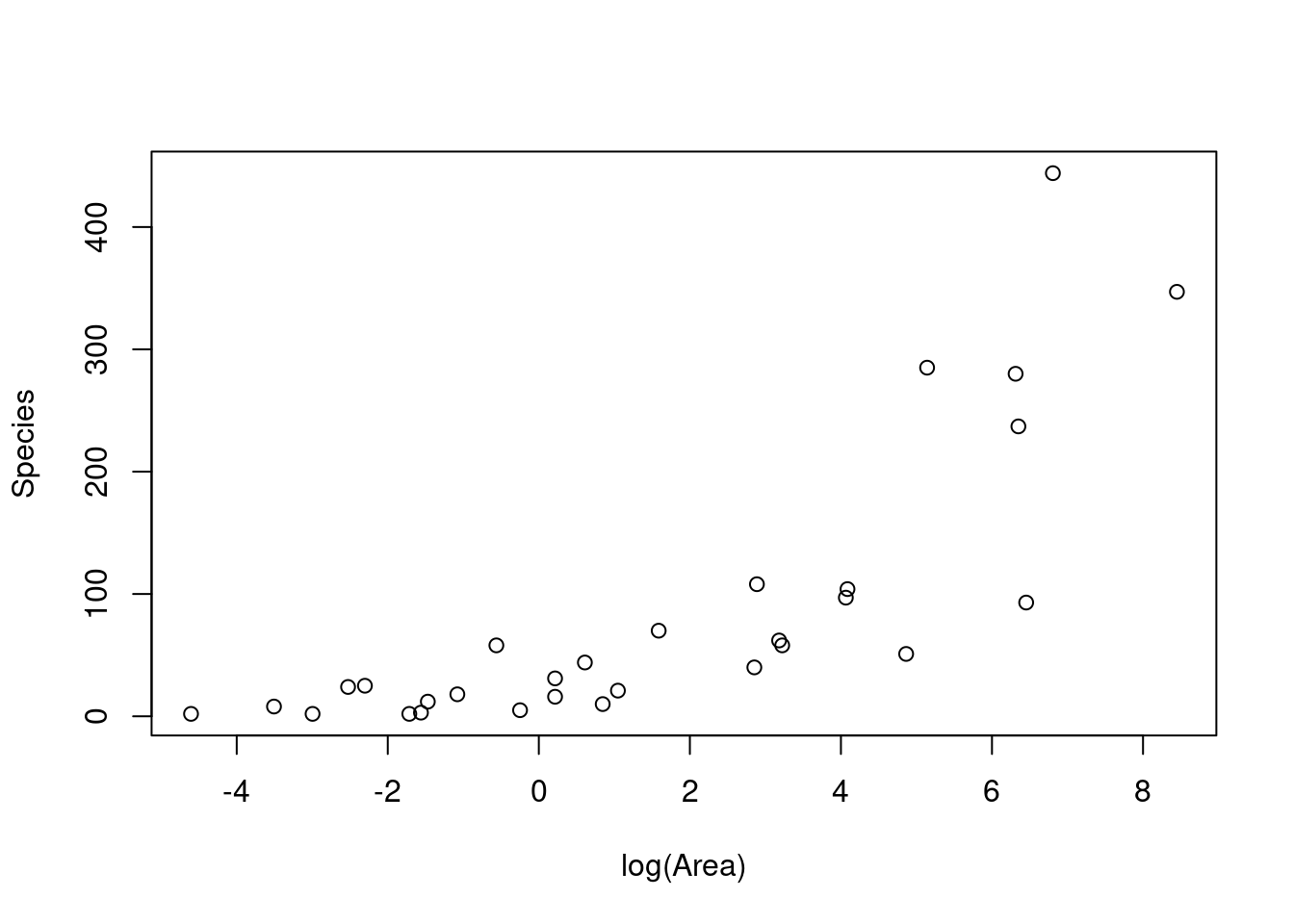
 plot(Species ~ log(Area), gala)

 hist(gala$Species)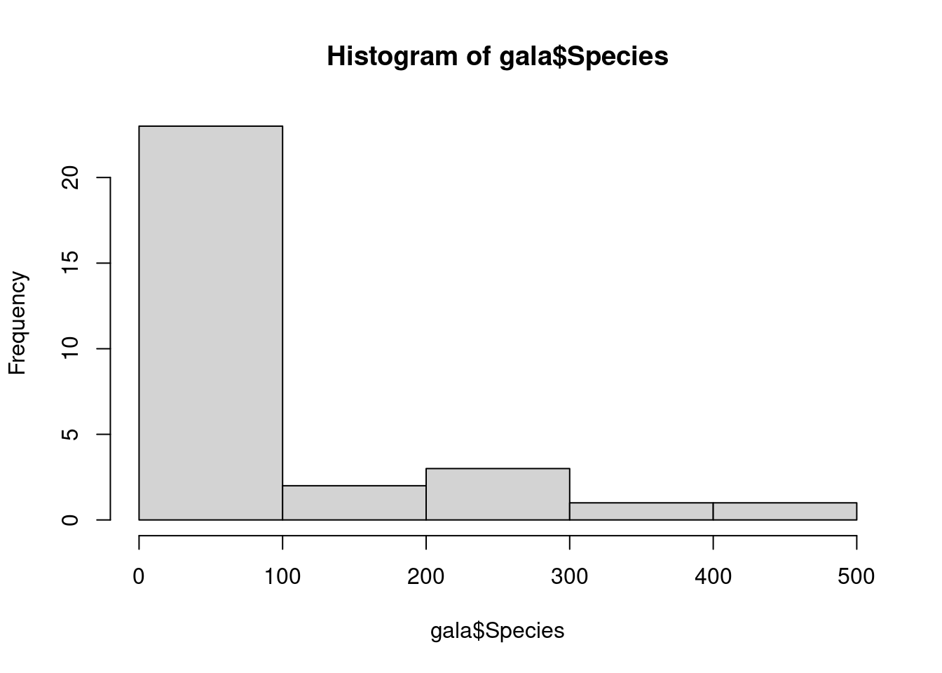

 modpl <- glm(Species ~ Area + Elevation + Nearest, family=poisson, gala)
res <- simulateResiduals(modpl)
testDispersion(res)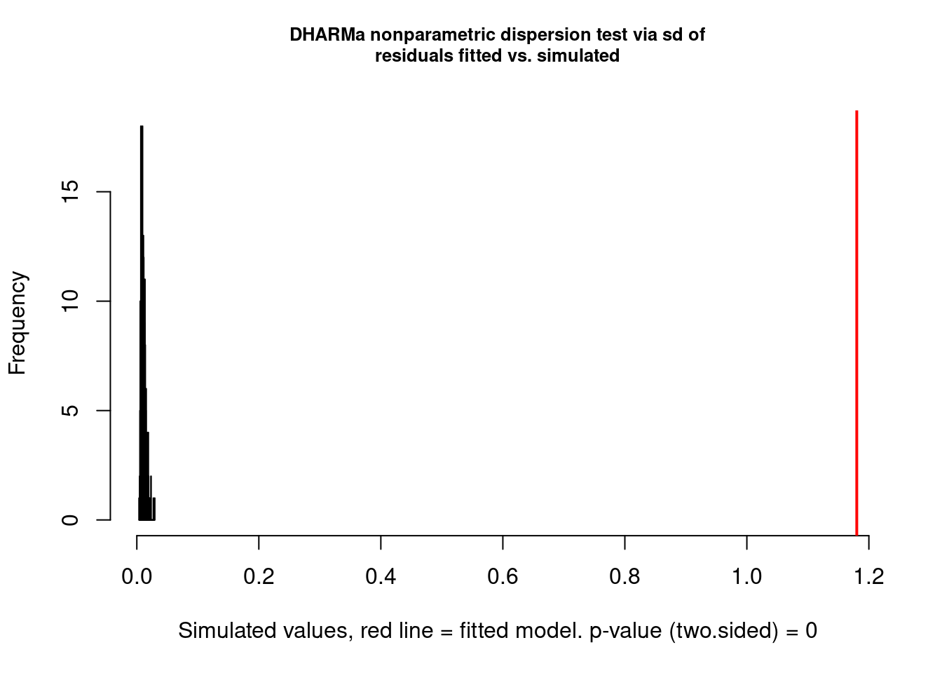


    DHARMa nonparametric dispersion test via sd of residuals fitted vs.
    simulated

data:  simulationOutput
dispersion = 110.32, p-value < 2.2e-16
alternative hypothesis: two.sided

testZeroInflation(res)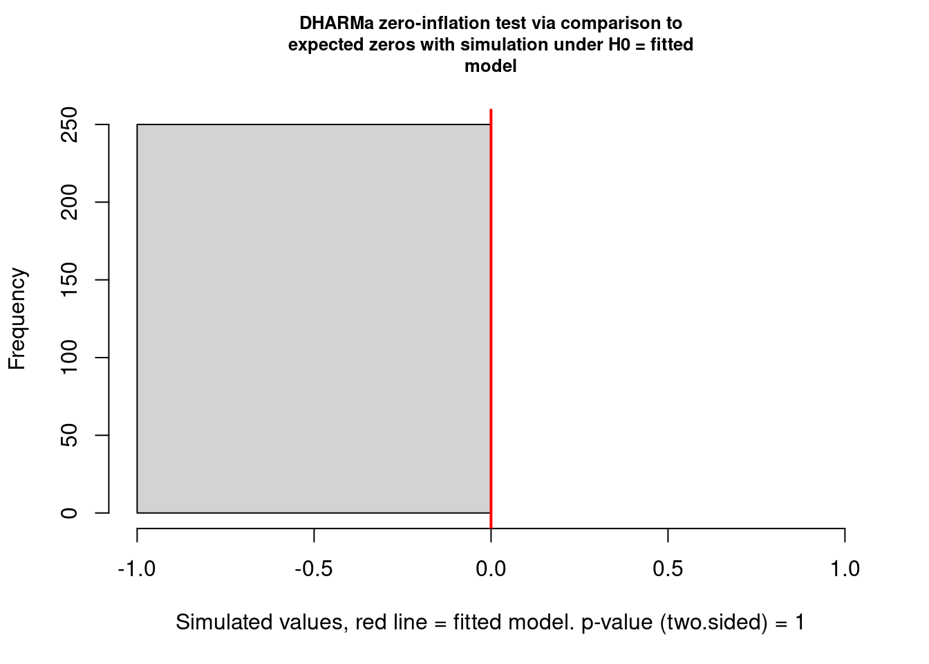


    DHARMa zero-inflation test via comparison to expected zeros with
    simulation under H0 = fitted model

data:  simulationOutput
ratioObsSim = NaN, p-value = 1
alternative hypothesis: two.sided

 mean(gala$Species)

[1] 85.23333

 var(gala$Species)

[1] 13140.74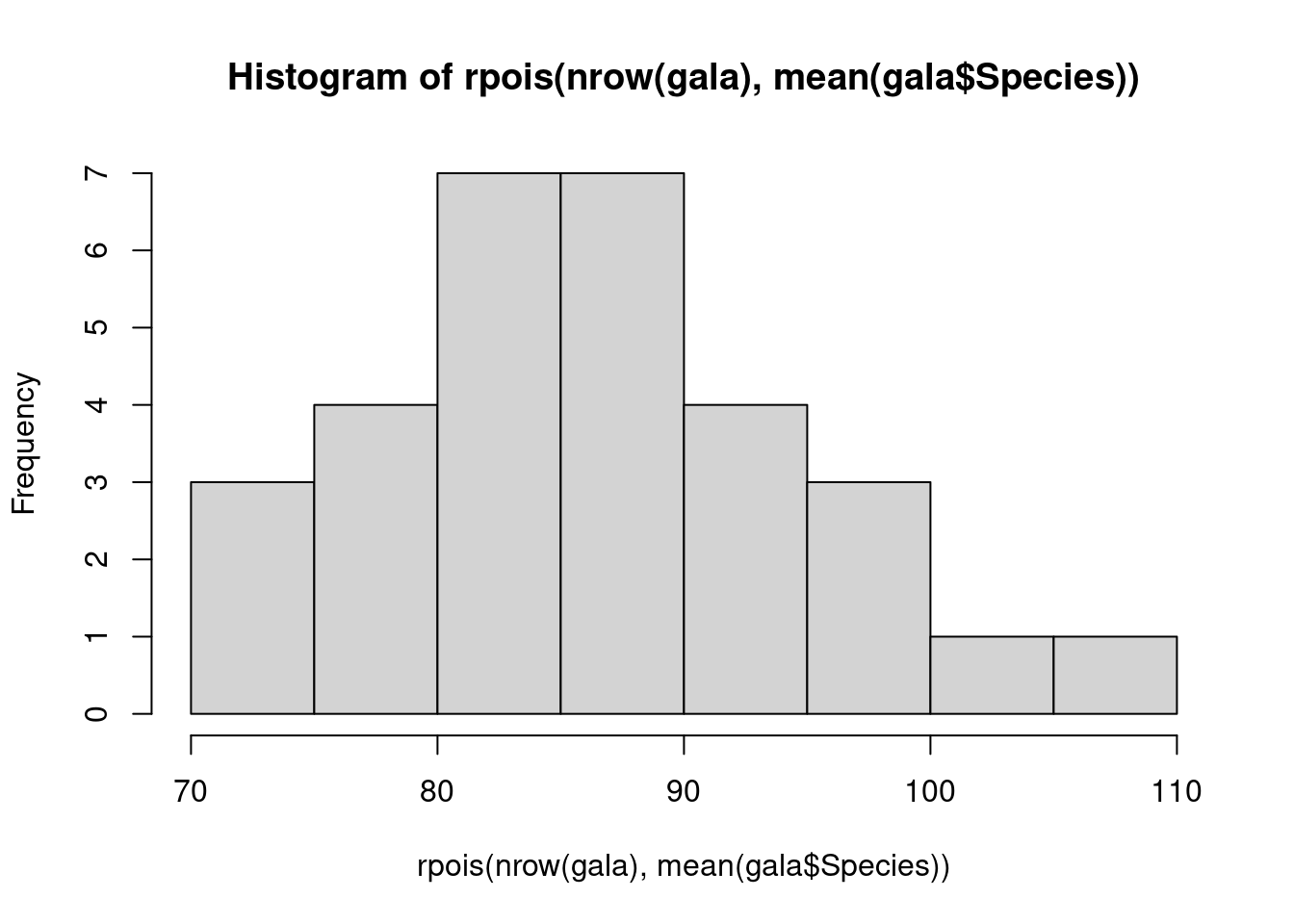

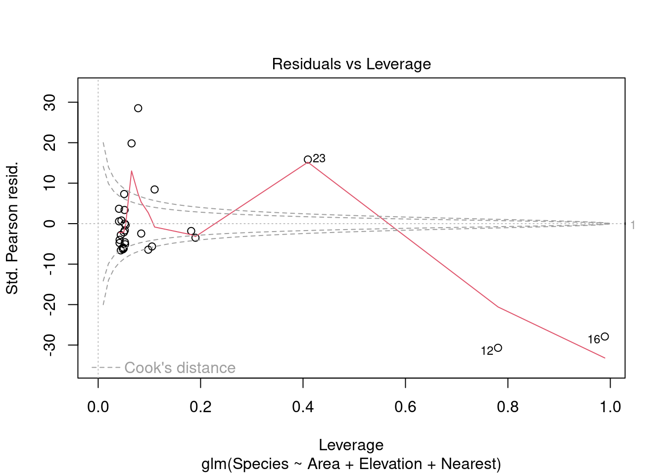
 hist(rpois(nrow(gala),mean(gala$Species)))

 plot(modpl)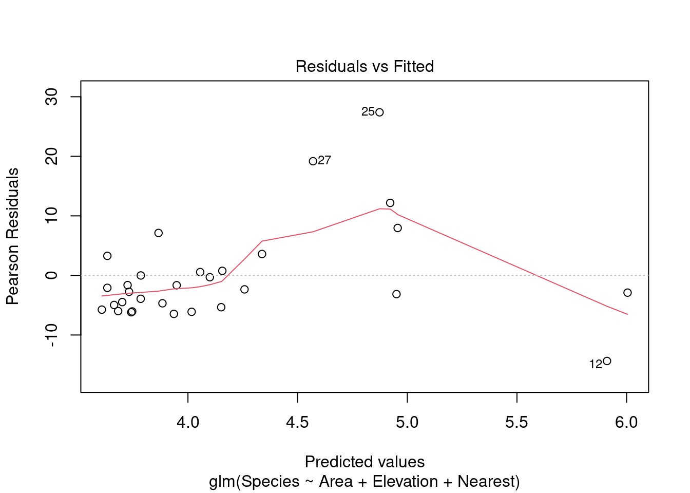

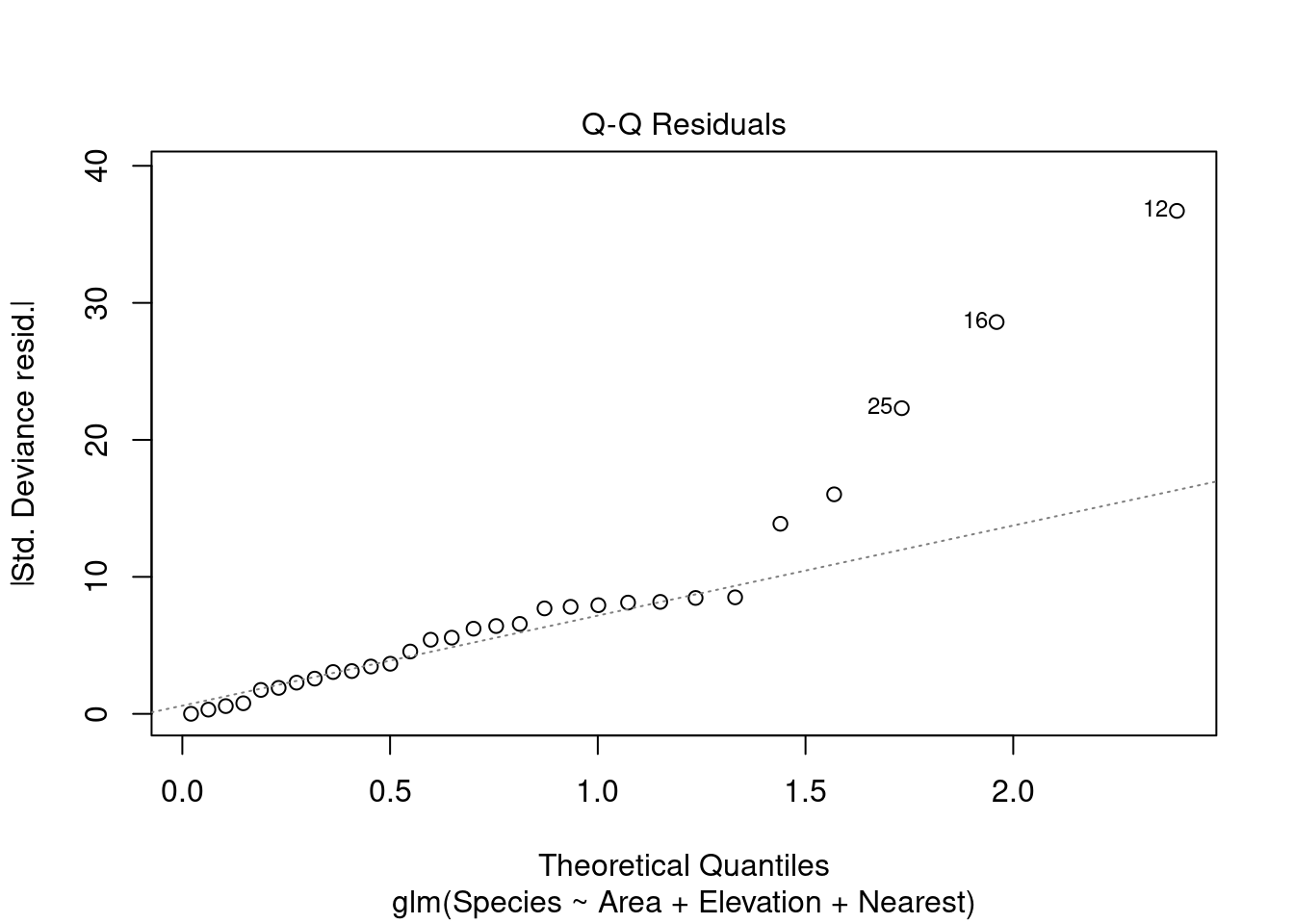
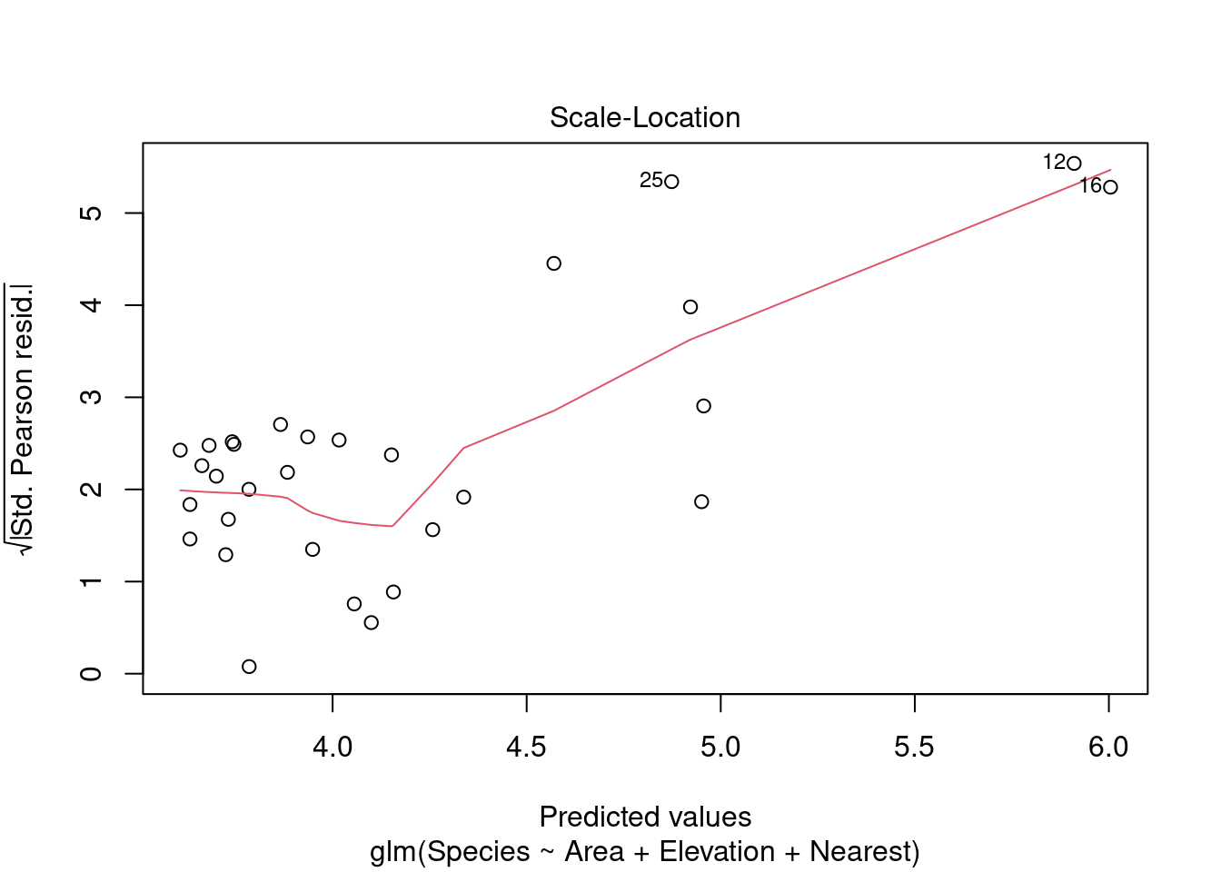
Warning in sqrt(crit * p * (1 - hh)/hh): NaNs produced
Warning in sqrt(crit * p * (1 - hh)/hh): NaNs produced