13  Multiple regression

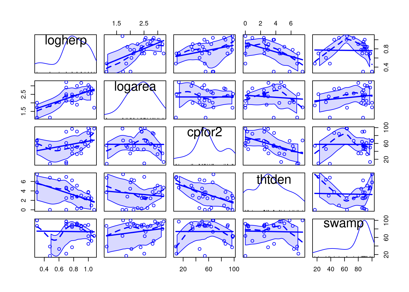
After completing this laboratory exercise, you should be able to:

• Use R to fit a multiple regression model, and compare the adequacy of several models using inferential and information theoretic criteria
• Use R to test hypotheses about the effects of different independent variables on the dependent variable of interest.
• Use R to evaluate multicollinearity among (supposedly) independent variables and its effects.
• Use R to do curvilinear (polynomial) regression.

13.1 R packages and data

For this lab you need:

• R packages:
  • ggplot2
  • car
  • lmtest
  • simpleboot
  • boot
  • MuMIn
• data files:
  • Mregdat.csv

13.2 Points to keep in mind

Multiple regression models are used in cases where there is one dependent variable and several independent, continuous variables. In many biological systems, the variable of interest may be influenced by several different factors, so that accurate description or prediction requires that several independent variables be included in the regression model. Before beginning, be aware that multiple regression takes time to learn well. Beginners should keep in mind several important points:

1. An overall regression model may be statistically significant even if none of the individual regression coefficients in the model are (caused by multicollinearity)
2. A multiple regression model may be “nonsignificant” even though some of the individual coefficients are “significant” (caused by overfitting)
3. Unless “independent” variables are uncorrelated in the sample, different model selection procedures may yield different results.

13.3 First look at the data

The file Mregdat.Rdata contains data collected in 30 wetlands in the Ottawa-Cornwall-Kingston area. The data included are

• the richness (number of species) of:
  • birds (bird , and its log transform logbird),
  • plants (plant, logpl),
  • mammals (mammal, logmam),
  • herptiles (herptile, logherp)
  • total species richness of all four groups combined (totsp, logtot)
• GPS coordinates of the wetland (lat , long)
• its area (logarea)
• the percentage of the wetland covered by water at all times during the year (swamp)
• the percentage of forested land within 1 km of the wetland (cpfor2)
• the density (in m/hectare) of hard-surface roads within 1 km of the wetland (thtden).

We will focus on herptiles for this exercise, so we better first have a look at how this variable is distributed and correlated to the potential independent variables:

mydata <- read.csv("data/Mregdat.csv")
scatterplotMatrix(
  ~ logherp + logarea + cpfor2 + thtden + swamp,
  regLine = TRUE, smooth = TRUE, diagonal = TRUE,
  data = mydata
)

Matrice de rélation et densité pour la richesse spécifique des amphibiens et reptiles

13.4 Multiple regression models from scratch

We begin the multiple regression exercise by considering a situation with one dependent variable and three (possibly) independent variables. First, we will start from scratch and build a multiple regression model based on what we know from building simple regression models. Next, we will look at automated methods of building multiple regressions models using simultaneous, forward, and backward stepwise procedures.

Exercise

Using the subset of the Mregdat.csv data file, regress logherp on logarea.

On the basis of the regression, what do you conclude?

model_loga <- lm(logherp ~ logarea, data = mydata)
summary(model_loga)

Call:
lm(formula = logherp ~ logarea, data = mydata)

Residuals:
     Min       1Q   Median       3Q      Max 
-0.38082 -0.09265  0.00763  0.10409  0.46977 

Coefficients:
            Estimate Std. Error t value Pr(>|t|)    
(Intercept)  0.18503    0.15725   1.177 0.249996    
logarea      0.24736    0.06536   3.784 0.000818 ***
---
Signif. codes:  0 '***' 0.001 '**' 0.01 '*' 0.05 '.' 0.1 ' ' 1

Residual standard error: 0.1856 on 26 degrees of freedom
  (2 observations deleted due to missingness)
Multiple R-squared:  0.3552,    Adjusted R-squared:  0.3304 
F-statistic: 14.32 on 1 and 26 DF,  p-value: 0.0008185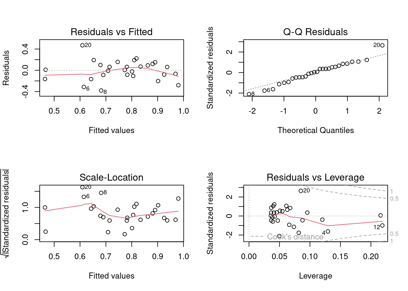

par(mfrow = c(2, 2))
plot(model_loga)

Checking model asusmptions for regression of logherp as a function of logarea

It looks like there is a positive relationship between herptile species richness and wetland area: the larger the wetland, the greater the number of species. Note, however, that about 2/3 of the observed variability in species richness among wetlands is not “explained” by wetland area (R² = 0.355). Residual analysis shows no major problems with normality, heteroscedasticity or independence of residuals.

Exercise

Rerun the above regression, this time replacing logarea with cpfor2 as the independent variable, such that the expression in the formula field reads: logherp ~ cpfor2 . What do you conclude?

Solution

model_logcp <- lm(logherp ~ cpfor2, data = mydata)
summary(model_logcp)

Call:
lm(formula = logherp ~ cpfor2, data = mydata)

Residuals:
     Min       1Q   Median       3Q      Max 
-0.49095 -0.10266  0.05881  0.16027  0.25159 

Coefficients:
            Estimate Std. Error t value Pr(>|t|)    
(Intercept) 0.609197   0.104233   5.845 3.68e-06 ***
cpfor2      0.002706   0.001658   1.632    0.115    
---
Signif. codes:  0 '***' 0.001 '**' 0.01 '*' 0.05 '.' 0.1 ' ' 1

Residual standard error: 0.2202 on 26 degrees of freedom
  (2 observations deleted due to missingness)
Multiple R-squared:  0.09289,   Adjusted R-squared:  0.058 
F-statistic: 2.662 on 1 and 26 DF,  p-value: 0.1148

According to this result, we would accept the null hypothesis, and conclude that there is no relationship between herptile density and the proportion of forest on adjacent lands. But what happens when we enter both variables into the regression simultaneously?

Exercise

Rerun the above regression one more time, this time adding both independent variables into the model at once, such that logherp ~ logarea + cpfor2 . What do you conclude?

Solution

model_mcp <- lm(logherp ~ logarea + cpfor2, data = mydata)
summary(model_mcp)

Call:
lm(formula = logherp ~ logarea + cpfor2, data = mydata)

Residuals:
     Min       1Q   Median       3Q      Max 
-0.40438 -0.11512  0.01774  0.08187  0.36179 

Coefficients:
            Estimate Std. Error t value Pr(>|t|)    
(Intercept) 0.027058   0.166749   0.162 0.872398    
logarea     0.247789   0.061603   4.022 0.000468 ***
cpfor2      0.002724   0.001318   2.067 0.049232 *  
---
Signif. codes:  0 '***' 0.001 '**' 0.01 '*' 0.05 '.' 0.1 ' ' 1

Residual standard error: 0.175 on 25 degrees of freedom
  (2 observations deleted due to missingness)
Multiple R-squared:  0.4493,    Adjusted R-squared:  0.4052 
F-statistic:  10.2 on 2 and 25 DF,  p-value: 0.0005774

Now we reject both null hypotheses that the slope of the regression of logherp on logarea is zero and that the slope of the regression of logherp on cpfor2 is zero.

Why is cpfor2 a significant predictor of logherp in the combined model when it was not significant in the simple linear model? The answer lies in the fact that it is sometimes necessary to control for one variable in order to detect the effect of another variable. In this case, there is a significant relationship between logherp and logarea that masks the relationship between logherp and cpfor2 . When both variables are entered into the model at once, the effect of logarea is controlled for, making it possible to detect a cpfor2 effect (and vice versa).

Exercise

Run another multiple regression, this time substituting thtden for cpfor2 as an independent variable (logherp ~ logarea + thtden).

Solution

model_mden <- lm(logherp ~ logarea + thtden, data = mydata)
summary(model_mden)

Call:
lm(formula = logherp ~ logarea + thtden, data = mydata)

Residuals:
     Min       1Q   Median       3Q      Max 
-0.31583 -0.12326  0.02095  0.13201  0.31674 

Coefficients:
            Estimate Std. Error t value Pr(>|t|)    
(Intercept)  0.37634    0.14926   2.521 0.018437 *  
logarea      0.22504    0.05701   3.947 0.000567 ***
thtden      -0.04196    0.01345  -3.118 0.004535 ** 
---
Signif. codes:  0 '***' 0.001 '**' 0.01 '*' 0.05 '.' 0.1 ' ' 1

Residual standard error: 0.1606 on 25 degrees of freedom
  (2 observations deleted due to missingness)
Multiple R-squared:  0.5358,    Adjusted R-squared:  0.4986 
F-statistic: 14.43 on 2 and 25 DF,  p-value: 6.829e-05

In this case we reject the null hypotheses that there are no effects of wetland area ( logarea ) and road density ( thtden ) on herptile richness ( logherp ). Note here that road density has a negative effect on richness, whereas wetland area and forested area ( cpfor2; results from previous regression) both have positive effects on herptile richness.

The R² of this model is even higher than the previous multiple regression model, reflecting a higher correlation between logherp and thtden than between logherp and cpfor2 (if you run a simple regression between logherp and thtden and compare it to the cpfor2 regression you should be able to detect this).

Thus far, it appears that herptile richness is related to wetland area ( logarea ), road density ( thtden ), and possibly forest cover on adjacent lands ( cpfor2 ). But, does it necessarily follow that if we build a regression model with all three independent variables, that all three will show significant relationships? No, because we have not yet examined the relationship between Logarea , cpfor2 and thtden . Suppose, for example, two of the variables (say, cpfor2 and thtden ) are perfectly correlated. Then the thtden effect is nothing more than the cpfor2 effect (and vice versa), so that once we include one or the other in the regression model, none of the remaining variability would be explained by the third variable.

Exercise

Fit a regression model with logherp as the dependent variable and logarea , cpfor2 and thtden as the independent variables. What do you conclude?

Solution

model_mtri <- lm(logherp ~ logarea + cpfor2 + thtden, data = mydata)
summary(model_mtri)

Call:
lm(formula = logherp ~ logarea + cpfor2 + thtden, data = mydata)

Residuals:
     Min       1Q   Median       3Q      Max 
-0.30729 -0.13779  0.02627  0.11441  0.29582 

Coefficients:
             Estimate Std. Error t value Pr(>|t|)    
(Intercept)  0.284765   0.191420   1.488 0.149867    
logarea      0.228490   0.057647   3.964 0.000578 ***
cpfor2       0.001095   0.001414   0.774 0.446516    
thtden      -0.035794   0.015726  -2.276 0.032055 *  
---
Signif. codes:  0 '***' 0.001 '**' 0.01 '*' 0.05 '.' 0.1 ' ' 1

Residual standard error: 0.1619 on 24 degrees of freedom
  (2 observations deleted due to missingness)
Multiple R-squared:  0.5471,    Adjusted R-squared:  0.4904 
F-statistic: 9.662 on 3 and 24 DF,  p-value: 0.0002291

Several things to note here:

1. The regression coefficient for cpfor2 has become non-significant: once the variability explained by logarea and thtden is removed, a non-significant part of the remaining variability is explained by cpfor2.
2. The R² for this model (.547 is only marginally larger than the R² for the model with only logarea and thtden (.536, which is again consistent with the non-significant coefficient for cpfor2.

Note also that although the regression coefficient for thtden has not changed much from that obtained when just thtden and logarea were included in the fitted model (-.036 vs -.042, the standard error for the regression coefficient for thtden has increased slightly, meaning the estimate is less precise. If the correlation between thtden and cpfor2 was greater, the change in precision would also be greater.

We can compare the fit of the last two models (i.e., the model with all 3 variables and the model with only logarea and thtden to decide which model is best to include.

anova(model_mtri, model_mden)

Analysis of Variance Table

Model 1: logherp ~ logarea + cpfor2 + thtden
Model 2: logherp ~ logarea + thtden
  Res.Df     RSS Df Sum of Sq     F Pr(>F)
1     24 0.62937                          
2     25 0.64508 -1 -0.015708 0.599 0.4465

Note that this is the identical result we obtained via the t-test of the effect of cpfor2 in the model with all 3 variables above as they are testing the same thing (this should make sense to you). From this analysis, we would conclude that the full model with all three variables included does not offer a significant improvement in fit over the model with only logarea and thtden. This isn’t surprising given that we already know that we cannot reject the null hypothesis of no effect of cpfor2 in the full model. Overall, we would conclude, on the basis of these analyses, that:

1. Given the three variables thtden , logarea and cpfor2 , the best model is one that includes the first two variables.
2. There is evidence of a negative relationship between herptile richness and the density of roads on adjacent lands.
3. There is evidence that the larger the wetland area, the greater the herptile species richness. Note that by “best”, I don’t mean the best possible model, I mean the best one given the three predictor variables we started with. It seems pretty clear that there are other factors controlling richness in wetlands, since even with the “best” model, almost half of the variability in richness is unexplained.

13.5 Stepwise multiple regression procedures

There are a number of techniques available for selecting the multiple regression model that best suits your data. When working with only three independent variables it is often sufficient to work through the different combinations of possible variables yourself, until you are satisfied you have fit the best model. This is, essentially, what we did in the first section of this lab. However, the process can become tedious when dealing with numerous independent variables, and you may find an automatic procedure for fitting models to be easier to work with.

Stepwise regression in R relies on the Akaike Information Criterion, as a measure of goodness of fit

\[AIC = 2k + 2ln(L))\]

where k is the number of regressors, and L is the maximized value of the likelihood function for the model). This is a statistic that rewards prediction precision while penalizing model complexity. If a new model has an AIC lower than that of the current model, the new model is a better fit to the data.

Exercise

Still working with the Mregdat data, run a stepwise multiple regression on the same set of variables:

# Stepwise Regression
step_mtri <- step(model_mtri, direction = "both")

Start:  AIC=-98.27
logherp ~ logarea + cpfor2 + thtden

          Df Sum of Sq     RSS     AIC
- cpfor2   1   0.01571 0.64508 -99.576
<none>                 0.62937 -98.267
- thtden   1   0.13585 0.76522 -94.794
- logarea  1   0.41198 1.04135 -86.167

Step:  AIC=-99.58
logherp ~ logarea + thtden

          Df Sum of Sq     RSS     AIC
<none>                 0.64508 -99.576
+ cpfor2   1   0.01571 0.62937 -98.267
- thtden   1   0.25092 0.89600 -92.376
- logarea  1   0.40204 1.04712 -88.013

step_mtri$anova # display results

      Step Df   Deviance Resid. Df Resid. Dev       AIC
1          NA         NA        24  0.6293717 -98.26666
2 - cpfor2  1 0.01570813        25  0.6450798 -99.57640

Examining the output, we find:

1. R calculated the AIC for the starting model (here the full model with the 3 independent variables.
2. The AIC for models where terms are deleted. Note here that the only way to reduce the AIC is to drop 2.
3. The AIC for models where terms are added or deleted from the model selected in the first step (i.e. logherp ~ logarea + thtden. Note that none of these models are better.

Instead of starting from the full (saturated) model and removing and possibly re-adding terms (i.e. direction = “both”), one can start from the null model and only add terms:

# Forward selection approach
model_null <- lm(logherp ~ 1, data = mydata)
step_f <- step(
  model_null,
  scope = ~ . + logarea + cpfor2 + thtden, direction = "forward"
)

Start:  AIC=-82.09
logherp ~ 1

          Df Sum of Sq    RSS     AIC
+ logarea  1   0.49352 0.8960 -92.376
+ thtden   1   0.34241 1.0471 -88.013
+ cpfor2   1   0.12907 1.2605 -82.820
<none>                 1.3895 -82.091

Step:  AIC=-92.38
logherp ~ logarea

         Df Sum of Sq     RSS     AIC
+ thtden  1   0.25093 0.64508 -99.576
+ cpfor2  1   0.13078 0.76522 -94.794
<none>                0.89600 -92.376

Step:  AIC=-99.58
logherp ~ logarea + thtden

         Df Sum of Sq     RSS     AIC
<none>                0.64508 -99.576
+ cpfor2  1  0.015708 0.62937 -98.267

step_f$anova # display results

       Step Df  Deviance Resid. Df Resid. Dev       AIC
1           NA        NA        27  1.3895281 -82.09073
2 + logarea -1 0.4935233        26  0.8960048 -92.37639
3  + thtden -1 0.2509250        25  0.6450798 -99.57640

You should first notice that the final result is the same as the default stepwise regression and as what we got building the model from scratch. In forward selection, R first fits the least complex model (i.e, with only an intercept), and then adds variables, one by one, according to AIC statistics. Thus, in the above example, the model was first fit with only an intercept. Next, logarea was added, followed by thtden. cpfor2 was not added because it would make AIC increase to above that of the model fit with the first two variables. Generally speaking, when doing multiple regressions, it is good practice to try several different methods (e.g. all regressions, stepwise, and backward elimination, etc.) and see whether you get the same results. If you don’t, then the “best” model may not be so obvious, and you will have to think very carefully about the inferences you draw. In this case, regardless of whether we use automatic, or forward/backward stepwise regression, we arrive at the same model.

When doing multiple regression, always bear in mind the following:

1. Different procedures may produce different “best” models, i.e. the “best” model obtained using forward stepwise regression needn’t necessarily be the same as that obtained using backward stepwise. It is good practice to try several different methods and see whether you end up with the same result. If you don’t, it is almost invariably due to multicollinearity among the independent variables.

2. Be wary of stepwise regression. As the authors of SYSTAT, another commonly used statistical package, note:

   Stepwise regression is probably the most abused computerized statistical technique ever devised. If you think you need automated stepwise regression to solve a particular problem, you probably don’t. Professional statisticians rarely use automated stepwise regression because it does not necessarily find the “best” fitting model, the “real” model, or alternative “plausible” models. Furthermore, the order in which variables enter or leave a stepwise program is usually of no theoretical significance. You are always better off thinking about why a model could generate your data and then testing that model.

3. Remember that just because there is a significant regression of Y on X doesn’t mean that X causes Y: correlation does not imply causation!

13.6 Detecting multicollinearity

Multicollinearity is the presence of correlations among independent variables. In extreme cases (perfect collinearity) it will prevent you from fitting some models.

Warning

When collinearity is not perfect, it reduces your ability to test for the effect of individual variables, but does not affect the ability of the model to predict.

The help file for the HH 📦package contains this clear passage about one of the indices of multicollinearity, the variance inflation factors:

A simple diagnostic of collinearity is the variance inflation factor, VIF one for each regression coefficient (other than the intercept). Since the condition of collinearity involves the predictors but not the response, this measure is a function of the X’s but not of Y. The VIF for predictor i is \[1/(1-R_i^2)\] where R_i² is the R² from a regression of predictor i against the remaining predictors. If R_i² is close to 1, this means that predictor i is well explained by a linear function of the remaining predictors, and, therefore, the presence of predictor i in the model is redundant. Values of VIF exceeding 5 are considered evidence of collinearity: The information carried by a predictor having such a VIF is contained in a subset of the remaining predictors. If, however, all of a model’s regression coefficients differ significantly from 0 (p-value < .05), a somewhat larger VIF may be tolerable.

VIFs indicate by how much the variance of each regression coefficient is increased by the presence of collinearity.

Note

There are several vif() functions (I know of at least three in the packages car, HH and DAAG) and I do not know if and how they differ.

To quantify multicollinarity, one can simply call the vif() function from the package car:

library(car)
vif(model_mtri)

 logarea   cpfor2   thtden 
1.022127 1.344455 1.365970 

Here there is no evidence that multicollinearity is a problem since all vif are close to 1.

13.7 Polynomial regression

In the regression models considered so far, we have assumed that the relationship between the dependent and independent variables is linear. If not, in some cases it can be made linear by transforming one or both variables. On the other hand, for many biological relationships no transformation in the world will help, and we are forced to go with some sort of non-linear regression method.

The simplest type of nonlinear regression method is polynomial regression, in which you fit regression models that include independent variables raised to some power greater than one, e.g. X², X³, etc.

Exercise

Plot the relationship between the residuals of the logherp ~ logarea regression and swamp.

Solution

# problème avec les données de manquantes dans logherp
mysub <- subset(mydata, !is.na(logherp))
# ajouter les résidus dans les donnée
mysub$resloga <- residuals(model_loga)
ggplot(data = mysub, aes(y = resloga, x = swamp)) +
  geom_point() +
  geom_smooth()

`geom_smooth()` using method = 'loess' and formula = 'y ~ x'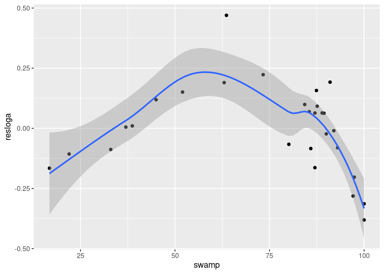

Relation entre swamp et les résidus de la régression entre logherp et logarea

Visual inspection of this graph suggests that there is a strong, but highly nonlinear, relationship between these two variables.

Exercise

Try regressing the residuals of the logherp ~ logarea regression on swamp. What do you conclude?

Solution

model_resloga <- lm(resloga ~ swamp, mysub)
summary(model_resloga)

Call:
lm(formula = resloga ~ swamp, data = mysub)

Residuals:
     Min       1Q   Median       3Q      Max 
-0.35088 -0.13819  0.00313  0.10849  0.45802 

Coefficients:
             Estimate Std. Error t value Pr(>|t|)
(Intercept)  0.084571   0.109265   0.774    0.446
swamp       -0.001145   0.001403  -0.816    0.422

Residual standard error: 0.1833 on 26 degrees of freedom
Multiple R-squared:  0.02498,   Adjusted R-squared:  -0.01252 
F-statistic: 0.666 on 1 and 26 DF,  p-value: 0.4219

In other words, the fit is terrible, even though you can see from the graph that there is in fact quite a strong relationship between the two - it’s just that it is a non-linear relationship. (If you look at model assumptions for this model, you will see strong evidence of nonlinearity, as expected) The pattern might be well described by a quadratic relation.

Exercise

Rerun the above regression but add a second term in the Formula field to represent swamp² . If you simply add swamp² in the model R won’t fit a quadratic effect, you need to use the functionI() which indicates that the formula within should be evaluated before fitting the model.

The expression should appear as:

\[ residuals ~ swamp + I(swamp^2)\].

What do you conclude? What does examination of the residuals from this multiple regression tell you?

Solution

model_resloga2 <- lm(resloga ~ swamp + I(swamp^2), mysub)
summary(model_resloga2)

Call:
lm(formula = resloga ~ swamp + I(swamp^2), data = mysub)

Residuals:
      Min        1Q    Median        3Q       Max 
-0.181185 -0.085350  0.007377  0.067327  0.242455 

Coefficients:
              Estimate Std. Error t value Pr(>|t|)    
(Intercept) -7.804e-01  1.569e-01  -4.975 3.97e-05 ***
swamp        3.398e-02  5.767e-03   5.892 3.79e-06 ***
I(swamp^2)  -2.852e-04  4.624e-05  -6.166 1.90e-06 ***
---
Signif. codes:  0 '***' 0.001 '**' 0.01 '*' 0.05 '.' 0.1 ' ' 1

Residual standard error: 0.1177 on 25 degrees of freedom
Multiple R-squared:  0.6132,    Adjusted R-squared:  0.5823 
F-statistic: 19.82 on 2 and 25 DF,  p-value: 6.972e-06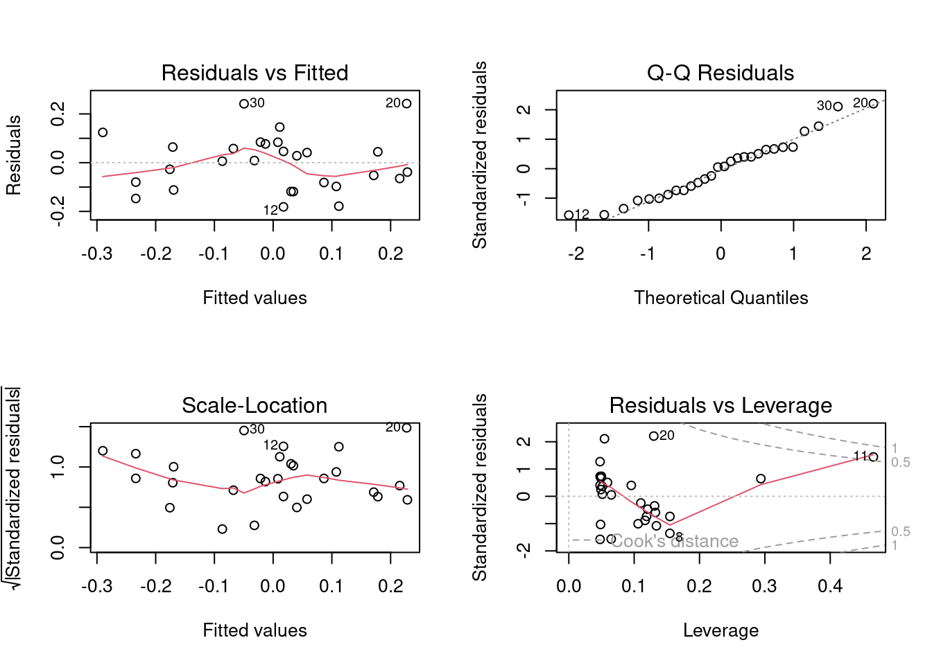

par(mfrow = c(2, 2))
plot(model_resloga2)

It is clear that once the effects of area are controlled for, a considerable amount of the remaining variability in herptile richness is explained by swamp , in a nonlinear fashion. If you examine model assumptions, you will see that compared to the linear model, the fit is much better.

Based on the results from the above analyses, how would you modify the regression model arrived at above? What, in your view, is the “best” overall model? Why? How would you rank the various factors in terms of their effects on herptile species richness?

In light of these results, we might want to try and fit a model which includes logarea, thtden, cpfor2, swamp and swamp^2^ :

Solution

model_poly1 <- lm(
  logherp ~ logarea + cpfor2 + thtden + swamp + I(swamp^2),
  data = mydata
)
summary(model_poly1)

Call:
lm(formula = logherp ~ logarea + cpfor2 + thtden + swamp + I(swamp^2), 
    data = mydata)

Residuals:
      Min        1Q    Median        3Q       Max 
-0.201797 -0.056170 -0.002072  0.051814  0.205626 

Coefficients:
              Estimate Std. Error t value Pr(>|t|)    
(Intercept) -3.203e-01  1.813e-01  -1.766   0.0912 .  
logarea      2.202e-01  3.893e-02   5.656 1.09e-05 ***
cpfor2      -7.864e-04  9.955e-04  -0.790   0.4380    
thtden      -2.929e-02  1.048e-02  -2.795   0.0106 *  
swamp        3.113e-02  5.898e-03   5.277 2.70e-05 ***
I(swamp^2)  -2.618e-04  4.727e-05  -5.538 1.45e-05 ***
---
Signif. codes:  0 '***' 0.001 '**' 0.01 '*' 0.05 '.' 0.1 ' ' 1

Residual standard error: 0.1072 on 22 degrees of freedom
  (2 observations deleted due to missingness)
Multiple R-squared:  0.8181,    Adjusted R-squared:  0.7767 
F-statistic: 19.78 on 5 and 22 DF,  p-value: 1.774e-07

Note that on the basis of this analysis, we could potentially drop cpfor2 and refit using the remaining variables:

Solution

model_poly2 <- lm(
  logherp ~ logarea + thtden + swamp + I(swamp^2),
  data = mydata
)
summary(model_poly2)

Call:
lm(formula = logherp ~ logarea + thtden + swamp + I(swamp^2), 
    data = mydata)

Residuals:
     Min       1Q   Median       3Q      Max 
-0.19621 -0.05444 -0.01202  0.07116  0.21295 

Coefficients:
              Estimate Std. Error t value Pr(>|t|)    
(Intercept) -3.461e-01  1.769e-01  -1.957   0.0626 .  
logarea      2.232e-01  3.842e-02   5.810 6.40e-06 ***
thtden      -2.570e-02  9.364e-03  -2.744   0.0116 *  
swamp        2.956e-02  5.510e-03   5.365 1.89e-05 ***
I(swamp^2)  -2.491e-04  4.409e-05  -5.649 9.46e-06 ***
---
Signif. codes:  0 '***' 0.001 '**' 0.01 '*' 0.05 '.' 0.1 ' ' 1

Residual standard error: 0.1063 on 23 degrees of freedom
  (2 observations deleted due to missingness)
Multiple R-squared:  0.8129,    Adjusted R-squared:  0.7804 
F-statistic: 24.98 on 4 and 23 DF,  p-value: 4.405e-08

How about multicollinearity in this model?

vif(model_poly2)

   logarea     thtden      swamp I(swamp^2) 
  1.053193   1.123491  45.845845  45.656453 

VIF for the two swamp terms are much higher than the standard threshold of 5. However, this is expected for polynomial terms, and not really a concern given that both terms are highly significant in the model. The high VIF means that these two coefficients are not estimated precisely, but using both in the model still allows to make a good prediction (i.e. account for the response to swamp).

13.8 Checking assumptions of a multiple regression model

All the model selection techniques or the manual model crafting assumes that the standard assumptions (independence, normality, homoscedasticity, linearity) are met. Given that a large number of models can be fitted, it may seem that testing the assumptions at each step would be an herculean task. However, it is generally sufficient to examine the residuals of the full (saturated) model and of the final model. Terms not contributing significantly to the fit do not affect residuals much, and therefore, the residuals to the full model, or the residuals to the final model, are generally sufficient.

Let’s have a look at the diagnostic plots for the final model. Here we use the check_model() function from the performance 📦.

Solution

library(performance)
check_model(model_poly2)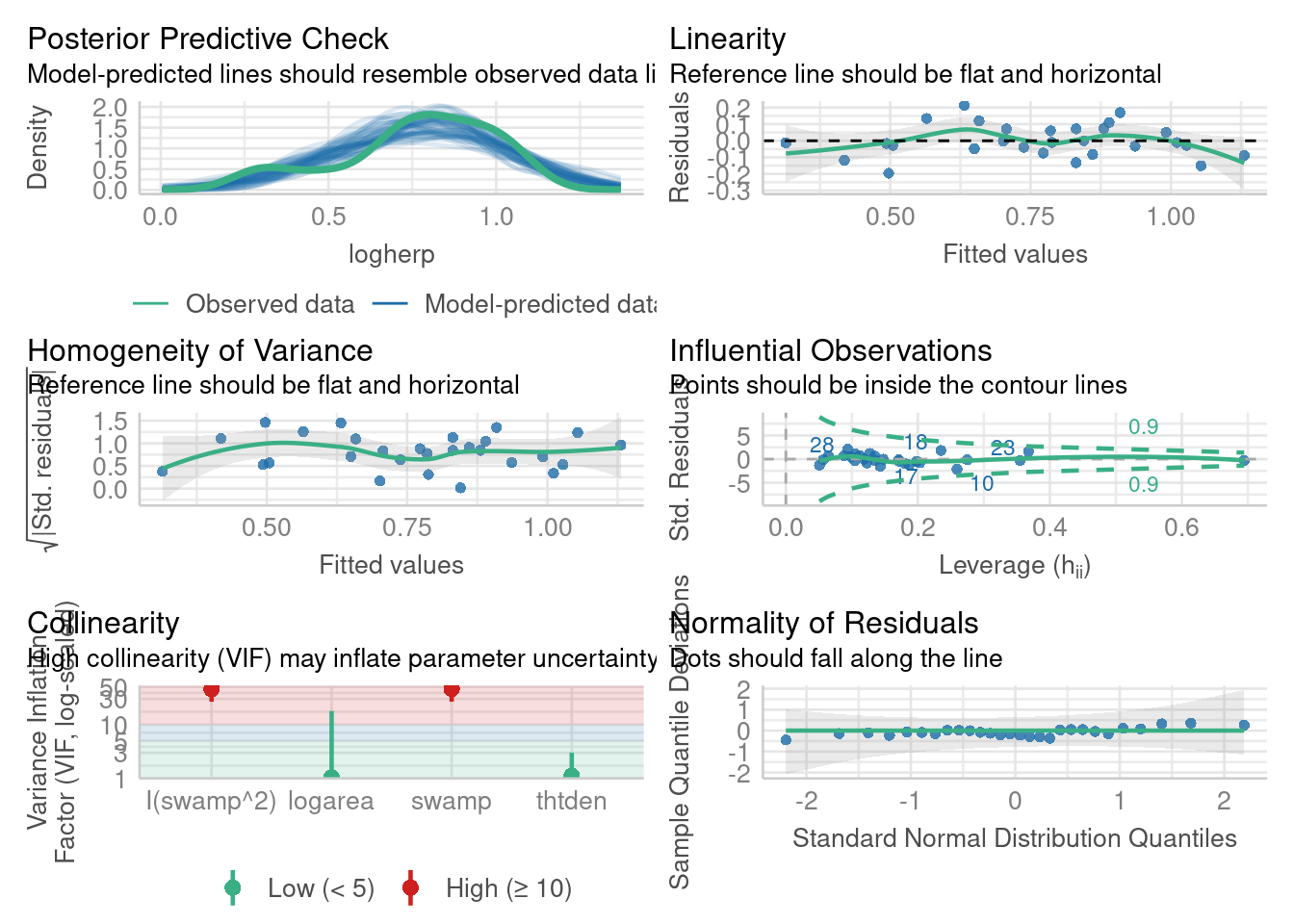

Conditions d’application du modèle model_poly2

Alternatively it can be done with the classic method

Code

par(mfrow = c(2, 2))
plot(model_poly2)

Conditions d’application du modèle model_poly2

Everything looks about right here. For the skeptic, let’s run the formal tests.

shapiro.test(residuals(model_poly2))

    Shapiro-Wilk normality test

data:  residuals(model_poly2)
W = 0.9837, p-value = 0.9278

The residuals do not deviate from normality. Good.

library(lmtest)
bptest(model_poly2)

    studentized Breusch-Pagan test

data:  model_poly2
BP = 3.8415, df = 4, p-value = 0.4279

No deviation from homoscedasticity either. Good.

dwtest(model_poly2)

    Durbin-Watson test

data:  model_poly2
DW = 1.725, p-value = 0.2095
alternative hypothesis: true autocorrelation is greater than 0

No serial correlation in the residuals, so no evidence of non-independence.

resettest(model_poly2, type = "regressor", data = mydata)

    RESET test

data:  model_poly2
RESET = 0.9823, df1 = 8, df2 = 15, p-value = 0.4859

And no significant deviation from linearity. So it seems that all is fine.

13.9 Visualizing effect size

How about effect size? How is that measured or viewed? The regression coefficients can be used to measure effect size, although it may be better to standardize them so that they become independent of measurement units. But a graph is often useful as well. In this context, some of the most useful graphs are called partial residual plots (or component + residual plots). These plots show how the dependent variable, corrected for other variables in the model, varies with each individual variable. Let’s have a look:

# Evaluate visually linearity and effect size
# component + residual plot
crPlots(model_poly2)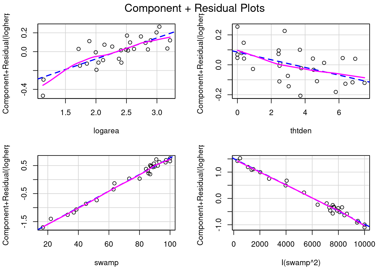

Graphiques de résidus partiels du modèle model_poly2

Note that the vertical scale varies among plots. For thtden, the dependent variable (log10(herptile richness)) varies by about 0.4 units over the range of thtden in the sample. For logarea, the variation is about 0.6 log units. For swamp, it is a bit tricky since there are two terms and they have opposite effect (leading to a peaked relationship), so the plots are less informative. However, there is no deviation from linearity to be seen.

To illustrate what these graphs would look like if there was deviation from linearity, let’s drop swamp² term and produce the graphs and run the RESET test

Solution

model_nopoly <- lm(
  logherp ~ logarea + thtden + swamp,
  data = mydata
)
crPlots(model_nopoly)

Graphiques de résidus partiels du modèle model_nopoly

The lack of linearity along the gradient of swamp becomes obvious. The RESET test also detects a violation from linearity:

resettest(model_nopoly, type = "regressor")

    RESET test

data:  model_nopoly
RESET = 6.7588, df1 = 6, df2 = 18, p-value = 0.0007066

13.10 Testing for interactions

When there are multiple independent variables one should always be ready to assess interactions. In most multiple regression contexts this is somewhat difficult because adding interaction terms increases overall multicollinearity and because in many cases there are not enough observations to test all interactions, or the observations are not well balanced to make powerful tests for interactions. Going back to our final model, see what happens if one tries to fit the fully saturated model with all interactions:

fullmodel_withinteractions <- lm(
  logherp ~ logarea * cpfor2 * thtden * swamp * I(swamp^2),
  data = mydata
)
summary(fullmodel_withinteractions)

Call:
lm(formula = logherp ~ logarea * cpfor2 * thtden * swamp * I(swamp^2), 
    data = mydata)

Residuals:
ALL 28 residuals are 0: no residual degrees of freedom!

Coefficients: (4 not defined because of singularities)
                                         Estimate Std. Error t value Pr(>|t|)
(Intercept)                            -5.948e+03        NaN     NaN      NaN
logarea                                 3.293e+03        NaN     NaN      NaN
cpfor2                                  7.080e+01        NaN     NaN      NaN
thtden                                  9.223e+02        NaN     NaN      NaN
swamp                                   1.176e+02        NaN     NaN      NaN
I(swamp^2)                             -3.517e-01        NaN     NaN      NaN
logarea:cpfor2                         -3.771e+01        NaN     NaN      NaN
logarea:thtden                         -4.781e+02        NaN     NaN      NaN
cpfor2:thtden                          -1.115e+01        NaN     NaN      NaN
logarea:swamp                          -7.876e+01        NaN     NaN      NaN
cpfor2:swamp                           -1.401e+00        NaN     NaN      NaN
thtden:swamp                           -1.920e+01        NaN     NaN      NaN
logarea:I(swamp^2)                      5.105e-01        NaN     NaN      NaN
cpfor2:I(swamp^2)                       3.825e-03        NaN     NaN      NaN
thtden:I(swamp^2)                       7.826e-02        NaN     NaN      NaN
swamp:I(swamp^2)                       -2.455e-03        NaN     NaN      NaN
logarea:cpfor2:thtden                   5.359e+00        NaN     NaN      NaN
logarea:cpfor2:swamp                    8.743e-01        NaN     NaN      NaN
logarea:thtden:swamp                    1.080e+01        NaN     NaN      NaN
cpfor2:thtden:swamp                     2.620e-01        NaN     NaN      NaN
logarea:cpfor2:I(swamp^2)              -5.065e-03        NaN     NaN      NaN
logarea:thtden:I(swamp^2)              -6.125e-02        NaN     NaN      NaN
cpfor2:thtden:I(swamp^2)               -1.551e-03        NaN     NaN      NaN
logarea:swamp:I(swamp^2)               -4.640e-04        NaN     NaN      NaN
cpfor2:swamp:I(swamp^2)                 3.352e-05        NaN     NaN      NaN
thtden:swamp:I(swamp^2)                 2.439e-04        NaN     NaN      NaN
logarea:cpfor2:thtden:swamp            -1.235e-01        NaN     NaN      NaN
logarea:cpfor2:thtden:I(swamp^2)        7.166e-04        NaN     NaN      NaN
logarea:cpfor2:swamp:I(swamp^2)                NA         NA      NA       NA
logarea:thtden:swamp:I(swamp^2)                NA         NA      NA       NA
cpfor2:thtden:swamp:I(swamp^2)                 NA         NA      NA       NA
logarea:cpfor2:thtden:swamp:I(swamp^2)         NA         NA      NA       NA

Residual standard error: NaN on 0 degrees of freedom
  (2 observations deleted due to missingness)
Multiple R-squared:      1, Adjusted R-squared:    NaN 
F-statistic:   NaN on 27 and 0 DF,  p-value: NA

Indeed, it is not possible to include all 32 terms with only 28 observations. There are not enough data points, R square is one, and the model perfectly overfits the data.

If you try to use an automated routine to “pick” the best model out of this soup, R complains:

step(fullmodel_withinteractions)

Error in step(fullmodel_withinteractions): AIC is -infinity for this model, so 'step' cannot proceed

Does this mean you can forget about potential interactions and simply accept the final model without a thought? No. You simply do not have enough data to test for all interactions. But there is a compromise worth attempting, comparing the final model to a model with a subset of the interactions, say all second order interactions, to check whether the inclusion of these interactions improves substantially the fit:

full_model_2ndinteractions <- lm(
  logherp ~ logarea + cpfor2 + thtden + swamp + I(swamp^2)
    + logarea:cpfor2
    + logarea:thtden
    + logarea:swamp
    + cpfor2:thtden
    + cpfor2:swamp
    + thtden:swamp,
  data = mydata
)
summary(full_model_2ndinteractions)

Call:
lm(formula = logherp ~ logarea + cpfor2 + thtden + swamp + I(swamp^2) + 
    logarea:cpfor2 + logarea:thtden + logarea:swamp + cpfor2:thtden + 
    cpfor2:swamp + thtden:swamp, data = mydata)

Residuals:
      Min        1Q    Median        3Q       Max 
-0.216880 -0.036534  0.003506  0.042990  0.175490 

Coefficients:
                 Estimate Std. Error t value Pr(>|t|)    
(Intercept)     4.339e-01  6.325e-01   0.686 0.502581    
logarea        -1.254e-01  2.684e-01  -0.467 0.646654    
cpfor2         -9.344e-03  7.205e-03  -1.297 0.213032    
thtden         -1.833e-01  9.035e-02  -2.028 0.059504 .  
swamp           3.569e-02  7.861e-03   4.540 0.000334 ***
I(swamp^2)     -3.090e-04  7.109e-05  -4.347 0.000500 ***
logarea:cpfor2  2.582e-03  2.577e-03   1.002 0.331132    
logarea:thtden  7.017e-02  3.359e-02   2.089 0.053036 .  
logarea:swamp  -5.290e-04  2.249e-03  -0.235 0.816981    
cpfor2:thtden  -2.095e-04  6.120e-04  -0.342 0.736544    
cpfor2:swamp    4.651e-05  5.431e-05   0.856 0.404390    
thtden:swamp    2.248e-04  4.764e-04   0.472 0.643336    
---
Signif. codes:  0 '***' 0.001 '**' 0.01 '*' 0.05 '.' 0.1 ' ' 1

Residual standard error: 0.108 on 16 degrees of freedom
  (2 observations deleted due to missingness)
Multiple R-squared:  0.8658,    Adjusted R-squared:  0.7735 
F-statistic: 9.382 on 11 and 16 DF,  p-value: 4.829e-05

This model fits the data slightly better than the “final” model (it explains 86.6% of the variance in logherp, compared to 81.2% for the “final” model without interactions), but has twice as many parameters.

If you look at the individual coefficients, some weird things happen: for example, the sign for logarea has changed. This is one of the symptoms of multicollinearity. Let’s look at the variance inflation factors:

vif(full_model_2ndinteractions)

there are higher-order terms (interactions) in this model
consider setting type = 'predictor'; see ?vif

       logarea         cpfor2         thtden          swamp     I(swamp^2) 
      49.86060       78.49622      101.42437       90.47389      115.08457 
logarea:cpfor2 logarea:thtden  logarea:swamp  cpfor2:thtden   cpfor2:swamp 
      66.97792       71.69894       67.27034       14.66814       29.41422 
  thtden:swamp 
      20.04410 

Ouch. All VIF are above 5, not only the ones involving the swamp terms. This model is not very satisfying it seems. Indeed the AIC for the two models indicate that the model with interactions has less information than the full model (remember, models with the lowest AIC value are to be preferred):

AIC(model_poly1)

[1] -38.3433

AIC(full_model_2ndinteractions)

[1] -34.86123

The anova() command can be used to test whether the addition of all interaction terms improves the fit significantly:

anova(model_poly1, full_model_2ndinteractions)

Analysis of Variance Table

Model 1: logherp ~ logarea + cpfor2 + thtden + swamp + I(swamp^2)
Model 2: logherp ~ logarea + cpfor2 + thtden + swamp + I(swamp^2) + logarea:cpfor2 + 
    logarea:thtden + logarea:swamp + cpfor2:thtden + cpfor2:swamp + 
    thtden:swamp
  Res.Df     RSS Df Sum of Sq      F Pr(>F)
1     22 0.25282                           
2     16 0.18651  6  0.066314 0.9481  0.489

This test indicates that the addition of interaction terms did not reduce significantly the residual variance around the full model. How about a comparison with the final model without cpfor2?

anova(model_poly2, full_model_2ndinteractions)

Analysis of Variance Table

Model 1: logherp ~ logarea + thtden + swamp + I(swamp^2)
Model 2: logherp ~ logarea + cpfor2 + thtden + swamp + I(swamp^2) + logarea:cpfor2 + 
    logarea:thtden + logarea:swamp + cpfor2:thtden + cpfor2:swamp + 
    thtden:swamp
  Res.Df     RSS Df Sum of Sq      F Pr(>F)
1     23 0.25999                           
2     16 0.18651  7  0.073486 0.9006 0.5294

And this comparison suggests that our final model does not make worse predictions than the full model with interactions.

13.11 Dredging and the information theoretical approach

One of the main critiques of stepwise methods is that the p-values are not strictly correct because of the large number of tests that are actually done. This is the multiple testing problem. In building linear models (multiple regression for example) from a large number of independent variables, and possibly their interactions, there are so many possible combinations that if one were to use Bonferroni type corrections, it would make tests very conservative.

An alternative, very elegantly advocated by Burnham and Anderson (2002, Model selection and multimodel inference: a practical information-theoretic approach. 2nd ed), is to use AIC (or better the AICc that is more appropriate for samples where the number of observations is less that about 40 times the number of variables) to rank potential models, and identify the set of models that are the best ones. One can then average the parameters across models, weighting using the probability that it is the best model to obtain coefficients that are more robust and less likely to be unduly affected by multicollinearity.

Warning

To compare models using AIC, models need to be fitted using the exact same data for each model. You thus need to be careful that there are no missing data when using an AIC based approach to model selection

The approach of comparing model fit using AIC was first developed to compare a set of model carefully build and chosen by the person doing the analysis based on a-priori knowledge and biological hypotheses. Some, however, developped an approach that I consider brainless and brutal to fit all potential models and then compare them using AIC. This approach has been implemented in the package MuMIn.

Note

I do not support the use of stepwise AIC or data dredging which are going against the philosophy of AIC and parsimony. Develop a model based on biological hypothesis and report all the results significant or not without dredging the data.

# redo the model double chekcing there are no "NA"
# specifying na.action

full_model_2ndinteractions <- update(
  full_model_2ndinteractions,
  . ~ .,
  data = mysub,
  na.action = "na.fail"
)

library(MuMIn)
dd <- dredge(full_model_2ndinteractions)

Fixed term is "(Intercept)"

Object dd will contain all possible models using the terms of our full model with 2nd order interactions. Then, we can have a look at the subset of models that have an AICc within 4 units from the lowest AICc model. (Burnham and Anderson suggest that models that deviate by more than 2 AICc units have very little empirical support):

# get models within 4 units of AICc from the best model
top_models_1 <- get.models(dd, subset = delta < 4)
avgmodel1 <- model.avg(top_models_1) # compute average parameters
summary(avgmodel1) # display averaged model

Call:
model.avg(object = top_models_1)

Component model call: 
lm(formula = logherp ~ <8 unique rhs>, data = mysub, na.action = 
     na.fail)

Component models: 
       df logLik   AICc delta weight
23457   7  27.78 -35.95  0.00   0.34
2345    6  25.78 -35.56  0.39   0.28
123457  8  28.30 -33.02  2.93   0.08
234578  8  28.26 -32.95  3.00   0.08
12345   7  26.17 -32.74  3.21   0.07
23458   7  26.06 -32.51  3.44   0.06
234567  8  27.88 -32.17  3.78   0.05
23456   7  25.79 -31.99  3.97   0.05

Term codes: 
        cpfor2     I(swamp^2)        logarea          swamp         thtden 
             1              2              3              4              5 
 logarea:swamp logarea:thtden   swamp:thtden 
             6              7              8 

Model-averaged coefficients:  
(full average) 
                 Estimate Std. Error Adjusted SE z value Pr(>|z|)    
(Intercept)    -2.075e-01  2.484e-01   2.593e-01   0.800    0.424    
logarea         1.314e-01  1.185e-01   1.222e-01   1.076    0.282    
swamp           3.193e-02  6.125e-03   6.438e-03   4.960    7e-07 ***
I(swamp^2)     -2.676e-04  4.904e-05   5.154e-05   5.193    2e-07 ***
thtden         -6.843e-02  5.324e-02   5.459e-02   1.254    0.210    
logarea:thtden  2.139e-02  2.506e-02   2.565e-02   0.834    0.404    
cpfor2         -1.202e-04  4.710e-04   4.886e-04   0.246    0.806    
swamp:thtden   -3.277e-05  1.419e-04   1.475e-04   0.222    0.824    
logarea:swamp   4.378e-05  5.378e-04   5.676e-04   0.077    0.939    
 
(conditional average) 
                 Estimate Std. Error Adjusted SE z value Pr(>|z|)    
(Intercept)    -2.075e-01  2.484e-01   2.593e-01   0.800   0.4236    
logarea         1.314e-01  1.185e-01   1.222e-01   1.076   0.2820    
swamp           3.193e-02  6.125e-03   6.438e-03   4.960    7e-07 ***
I(swamp^2)     -2.676e-04  4.904e-05   5.154e-05   5.193    2e-07 ***
thtden         -6.843e-02  5.324e-02   5.459e-02   1.254   0.2100    
logarea:thtden  3.924e-02  2.125e-02   2.251e-02   1.743   0.0813 .  
cpfor2         -8.187e-04  9.692e-04   1.027e-03   0.797   0.4253    
swamp:thtden   -2.402e-04  3.127e-04   3.313e-04   0.725   0.4684    
logarea:swamp   4.462e-04  1.664e-03   1.762e-03   0.253   0.8001    
---
Signif. codes:  0 '***' 0.001 '**' 0.01 '*' 0.05 '.' 0.1 ' ' 1

confint(avgmodel1) # display CI for averaged coefficients

                       2.5 %        97.5 %
(Intercept)    -0.7157333646  0.3007147516
logarea        -0.1080048582  0.3708612563
swamp           0.0193158426  0.0445532538
I(swamp^2)     -0.0003686653 -0.0001666418
thtden         -0.1754184849  0.0385545120
logarea:thtden -0.0048800385  0.0833595106
cpfor2         -0.0028313465  0.0011940283
swamp:thtden   -0.0008894138  0.0004090457
logarea:swamp  -0.0030067733  0.0038991294

1. components models: You first get the list of the models with an AICc within the desired 4 units of the best model. The variables that are included in the model are coded with the key just below.
2. For each model, in addition to the AICc, the Akaike weights are calculated. They represent the relative likelihood of a model, and indicate the relative importance of a model compared to the other models tested.
3. Mode-averaged coefficients: For the subset of models, weighted averages (using Akaike weights) for model parameters are calculated, with 95% CI. Note that, by default, terms missing from a model are assumed to have a coefficient of 0.

13.12 Bootstrapping multiple regression

When data do not meet the assumptions of normality and homoscedasticity and it is not possible to transform the data to meet the assumptions, bootstraping can be used to compute confidence intervals for coefficients. If the distribution of the bootstrapped coefficients is symmetrical and approximately Gaussian, then empirical percentiles can be used to estimate the confidence limits.

The following code, using the simpleboot 📦 has been designed to be easily modifiable and will compute CI using empirical percentiles. Following this is an easier approach using the library boot that will calculate several different bootstrap confidence limits.

############################################################
#######
# Bootstrap analysis the simple way with library simpleboot
# Define model to be bootstrapped and the data source used
mymodel <- lm(logherp ~ logarea + thtden + swamp + I(swamp^2), data = mydata)
# Set the number of bootstrap iterations
nboot <- 1000
library(simpleboot)
# R is the number of bootstrap iterations
# Setting rows to FALSE indicates resampling of residuals
mysimpleboot <- lm.boot(mymodel, R = nboot, rows = FALSE)
# Extract bootstrap coefficients
myresults <- sapply(mysimpleboot$boot.list, function(x) x$coef)
# Transpose matrix so that lines are bootstrap iterations
# and columns are coefficients
tmyresults <- t(myresults)

You can then plot the results using the follwoing code. When run, it will pause to let you have a look at the distribution for each coefficient in the model by producing plots like:

# Plot histograms of bootstrapped coefficients
ncoefs <- length(data.frame(tmyresults))
par(mfrow = c(1, 2), mai = c(0.5, 0.5, 0.5, 0.5), ask = TRUE)
for (i in 1:ncoefs) {
  lab <- colnames(tmyresults)[i]
  x <- tmyresults[, i]
  plot(density(x), main = lab, xlab = "")
  abline(v = mymodel$coef[i], col = "red")
  abline(v = quantile(x, c(0.025, 0.975)))
  hist(x, main = lab, xlab = "")
  abline(v = quantile(x, c(0.025, 0.975)))
  abline(v = mymodel$coef[i], col = "red")
}

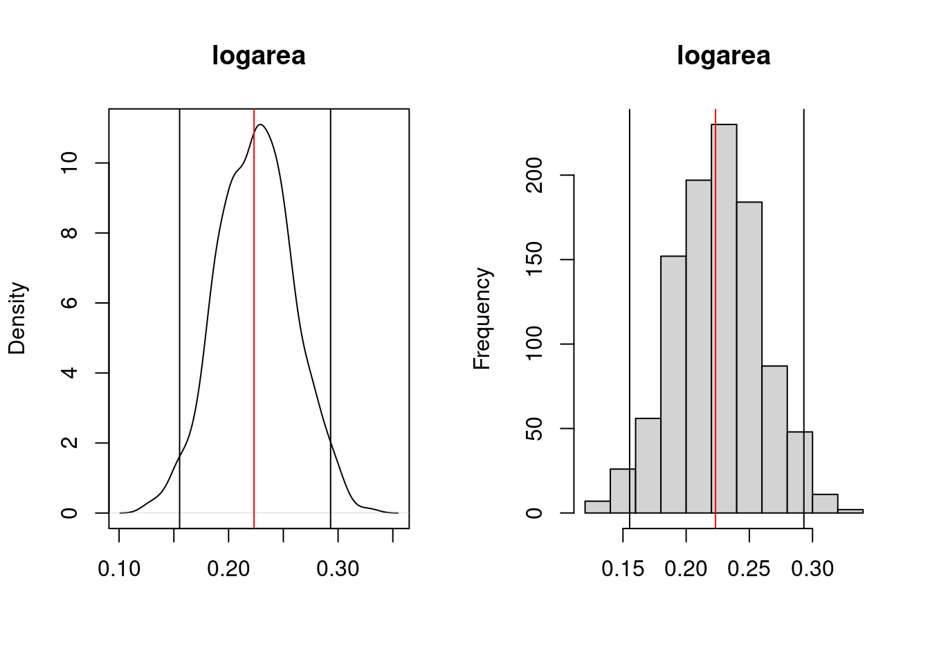
Distribution of bootstrapped estimates for logarea

The top plot is the probability density function and the bottom one is the histogram of the bootstrap estimates for the coefficient. On these plots, the red line indicate the value of the parameter in the ordinary analysis, and the two vertical black lines mark the limits of the 95% confidence interval. Here the CI does not include 0 and one can conclude that the effect of logarea on logherp is significantly positive.

Precise values for the limits can be obtained by:

# Display empirical bootstrap quantiles (not corrected for bias)
p <- c(0.005, 0.01, 0.025, 0.05, 0.95, 0.975, 0.99, 0.995)
apply(tmyresults, 2, quantile, p)

       (Intercept)   logarea       thtden      swamp    I(swamp^2)
0.5%  -0.703337469 0.1372880 -0.045562085 0.01704499 -0.0003491593
1%    -0.682330238 0.1437596 -0.044178131 0.01765760 -0.0003417409
2.5%  -0.634774104 0.1552722 -0.040448896 0.01992423 -0.0003262314
5%    -0.598948564 0.1692405 -0.038330203 0.02156104 -0.0003135141
95%   -0.097107227 0.2829351 -0.011854745 0.03770433 -0.0001839501
97.5% -0.064126662 0.2931585 -0.010018307 0.03946455 -0.0001712404
99%   -0.007850978 0.3021190 -0.007672276 0.04064188 -0.0001547049
99.5%  0.031935680 0.3061687 -0.004818113 0.04145426 -0.0001500559

These confidence limits are not reliable when the distribution of the bootstrap estimates deviate from Gaussian. If they do,, then it is preferable to compute so-called bias-corrected accelerated (BCa) confidence limits. The following code does just that:

################################################
# Bootstrap analysis in multiple regression with BCa confidence intervals
# Preferable when parameter distribution is far from normal
# Bootstrap 95% BCa CI for regression coefficients

library(boot)
# function to obtain regression coefficients for each iteration
bs <- function(formula, data, indices) {
  d <- data[indices, ] # allows boot to select sample
  fit <- lm(formula, data = d)
  return(coef(fit))
}
# bootstrapping with 1000 replications
results <- boot(
  data = mydata, statistic = bs, R = 1000,
  formula = logherp ~ logarea + thtden + swamp + I(swamp^2)
)
# view results

To get teh results, the following code will produce the standard graph for each coefficient and the resulting BCa interval.

plot(results, index = 1) # intercept
plot(results, index = 2) # logarea
plot(results, index = 3) # thtden
plot(results, index = 4) # swamp
plot(results, index = 5) # swamp2

# get 95% confidence intervals
boot.ci(results, type = "bca", index = 1)
boot.ci(results, type = "bca", index = 2)
boot.ci(results, type = "bca", index = 3)
boot.ci(results, type = "bca", index = 4)
boot.ci(results, type = "bca", index = 5)

For logarea, we get:

BOOTSTRAP CONFIDENCE INTERVAL CALCULATIONS
Based on 1000 bootstrap replicates

CALL : 
boot.ci(boot.out = results, type = "bca", index = 2)

Intervals : 
Level       BCa          
95%   ( 0.1185,  0.3176 )  
Calculations and Intervals on Original Scale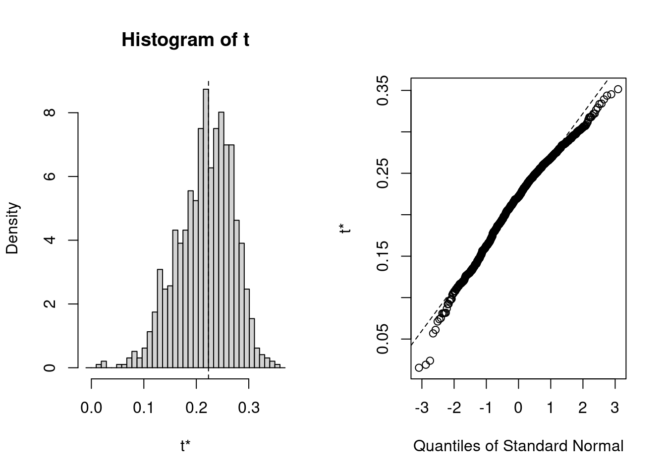

Note that the BCa interval is from 0.12 to 0.32, whereas the simpler percentile interval is 0.16 to 0.29. BCa interval here is longer on the low side, and shorter on the high side, which it should be given the distribution of bootstrap estimates.

13.13 Permutation test

Permutation tests are more rarely performed in multiple regression contexts than bootstrap. But here is code to do it.

############################################################
##########
# Permutation in multiple regression
#
# using lmperm library
library(lmPerm)
# Fit desired model on the desired dataframe
my_model <- lm(logherp ~ logarea + thtden + swamp + I(swamp^2),
  data = mydata
)
my_model_prob <- lmp(
  logherp ~ logarea + thtden + swamp + I(swamp^2),
  data = mydata, perm = "Prob"
)
summary(my_model)
summary(my_model_prob)